By Salerno | December 23, 2019
Random Forest
In this post we will explore some ideas around the Random Forest model
Objective
We are working on in the dataset called Boston Housing and the main idea here is regression task and we are concerned with modeling the price of houses in thousands of dollars in the Surburb of Boston.
So, we are dirting our hands in a regression predictive modeling problem.
The main goal here is to fit a regression model that best explains the variation in medv variable.
Data
In terms of dataset, we are using a file from UCI and their content is related of Housing Values in Suburbs of Boston.
# to get the data
BHData <- read.table(url("https://archive.ics.uci.edu/ml/machine-learning-databases/housing/housing.data"), sep = "")
For our study we are working on 506 rows (events) and 14 columns. One of them called medv is our target value - y or response variable.
# knowing the dimension of the data
dim(BHData)
## [1] 506  14
Set names of the dataset
# changing the variable's names
names(BHData)<- c("crim","zn","indus","chas","nox","rm",
       "age","dis","rad","tax","ptratio","black","lstat","medv")
EDA (Exploratory Data Analysis)
Usually as a first task, we use some Exploratory Data Analysis to understand how the data is distributed and extract preliminary knowledge.
# structure
str(BHData)
## 'data.frame':    506 obs. of  14 variables:
##  $ crim   : num  0.00632 0.02731 0.02729 0.03237 0.06905 ...
##  $ zn     : num  18 0 0 0 0 0 12.5 12.5 12.5 12.5 ...
##  $ indus  : num  2.31 7.07 7.07 2.18 2.18 2.18 7.87 7.87 7.87 7.87 ...
##  $ chas   : int  0 0 0 0 0 0 0 0 0 0 ...
##  $ nox    : num  0.538 0.469 0.469 0.458 0.458 0.458 0.524 0.524 0.524 0.524 ...
##  $ rm     : num  6.58 6.42 7.18 7 7.15 ...
##  $ age    : num  65.2 78.9 61.1 45.8 54.2 58.7 66.6 96.1 100 85.9 ...
##  $ dis    : num  4.09 4.97 4.97 6.06 6.06 ...
##  $ rad    : int  1 2 2 3 3 3 5 5 5 5 ...
##  $ tax    : num  296 242 242 222 222 222 311 311 311 311 ...
##  $ ptratio: num  15.3 17.8 17.8 18.7 18.7 18.7 15.2 15.2 15.2 15.2 ...
##  $ black  : num  397 397 393 395 397 ...
##  $ lstat  : num  4.98 9.14 4.03 2.94 5.33 ...
##  $ medv   : num  24 21.6 34.7 33.4 36.2 28.7 22.9 27.1 16.5 18.9 ...
As you can see using the summary() function below, there are variables with different ranges. It is could badly impact the response variable if we have had a less numeric range between each of the predictors variables.
As we have to improve the predictive accuracy of our model we have not allowed that this large difference in the range of variables impact the accuracy of the predicting task upon the medv variable.
You will see the adequate treatment in the Pre-processing topic.
summary(BHData)
##       crim                zn             indus            chas
##  Min.   : 0.00632   Min.   :  0.00   Min.   : 0.46   Min.   :0.00000
##  1st Qu.: 0.08204   1st Qu.:  0.00   1st Qu.: 5.19   1st Qu.:0.00000
##  Median : 0.25651   Median :  0.00   Median : 9.69   Median :0.00000
##  Mean   : 3.61352   Mean   : 11.36   Mean   :11.14   Mean   :0.06917
##  3rd Qu.: 3.67708   3rd Qu.: 12.50   3rd Qu.:18.10   3rd Qu.:0.00000
##  Max.   :88.97620   Max.   :100.00   Max.   :27.74   Max.   :1.00000
##       nox               rm             age              dis
##  Min.   :0.3850   Min.   :3.561   Min.   :  2.90   Min.   : 1.130
##  1st Qu.:0.4490   1st Qu.:5.886   1st Qu.: 45.02   1st Qu.: 2.100
##  Median :0.5380   Median :6.208   Median : 77.50   Median : 3.207
##  Mean   :0.5547   Mean   :6.285   Mean   : 68.57   Mean   : 3.795
##  3rd Qu.:0.6240   3rd Qu.:6.623   3rd Qu.: 94.08   3rd Qu.: 5.188
##  Max.   :0.8710   Max.   :8.780   Max.   :100.00   Max.   :12.127
##       rad              tax           ptratio          black
##  Min.   : 1.000   Min.   :187.0   Min.   :12.60   Min.   :  0.32
##  1st Qu.: 4.000   1st Qu.:279.0   1st Qu.:17.40   1st Qu.:375.38
##  Median : 5.000   Median :330.0   Median :19.05   Median :391.44
##  Mean   : 9.549   Mean   :408.2   Mean   :18.46   Mean   :356.67
##  3rd Qu.:24.000   3rd Qu.:666.0   3rd Qu.:20.20   3rd Qu.:396.23
##  Max.   :24.000   Max.   :711.0   Max.   :22.00   Max.   :396.90
##      lstat            medv
##  Min.   : 1.73   Min.   : 5.00
##  1st Qu.: 6.95   1st Qu.:17.02
##  Median :11.36   Median :21.20
##  Mean   :12.65   Mean   :22.53
##  3rd Qu.:16.95   3rd Qu.:25.00
##  Max.   :37.97   Max.   :50.00
Pre-processing
Remove outliers
#cut-off values are given by the formal definition of an outlier:
#Q3 + 1.5*IQR
upper_cut_off1 <- (quantile(BHData$crim, 0.75)) + (IQR(BHData$crim))*1.5
upper_cut_off1
##      75%
## 9.069639


upper_cut_off2 <- (quantile(BHData$zn, 0.75)) + (IQR(BHData$zn))*1.5
upper_cut_off2
##   75%
## 31.25


upper_cut_off3 <- (quantile(BHData$indus, 0.75)) + (IQR(BHData$indus))*1.5
upper_cut_off3
##    75%
## 37.465


upper_cut_off4 <- (quantile(BHData$chas, 0.75)) + (IQR(BHData$chas))*1.5
upper_cut_off4
## 75%
##   0
Feature Scaling
It is an important step called featured scaling to get all the data scaled in the range [0,1]. This method has chosen can be called as well as normalization.
# calculating the maximun in each column
max_data <- apply(BHData, 2, max)
# calculating the minimun in each column
min_data <- apply(BHData, 2, min)# applying the normalization
BHDataScaled <- as.data.frame(scale(BHData,center = min_data,
scale = max_data - min_data))To confirm normalization process:
summary(BHDataScaled)
##       crim                 zn             indus             chas
##  Min.   :0.0000000   Min.   :0.0000   Min.   :0.0000   Min.   :0.00000
##  1st Qu.:0.0008511   1st Qu.:0.0000   1st Qu.:0.1734   1st Qu.:0.00000
##  Median :0.0028121   Median :0.0000   Median :0.3383   Median :0.00000
##  Mean   :0.0405441   Mean   :0.1136   Mean   :0.3914   Mean   :0.06917
##  3rd Qu.:0.0412585   3rd Qu.:0.1250   3rd Qu.:0.6466   3rd Qu.:0.00000
##  Max.   :1.0000000   Max.   :1.0000   Max.   :1.0000   Max.   :1.00000
##       nox               rm              age              dis
##  Min.   :0.0000   Min.   :0.0000   Min.   :0.0000   Min.   :0.00000
##  1st Qu.:0.1317   1st Qu.:0.4454   1st Qu.:0.4338   1st Qu.:0.08826
##  Median :0.3148   Median :0.5073   Median :0.7683   Median :0.18895
##  Mean   :0.3492   Mean   :0.5219   Mean   :0.6764   Mean   :0.24238
##  3rd Qu.:0.4918   3rd Qu.:0.5868   3rd Qu.:0.9390   3rd Qu.:0.36909
##  Max.   :1.0000   Max.   :1.0000   Max.   :1.0000   Max.   :1.00000
##       rad              tax            ptratio           black
##  Min.   :0.0000   Min.   :0.0000   Min.   :0.0000   Min.   :0.0000
##  1st Qu.:0.1304   1st Qu.:0.1756   1st Qu.:0.5106   1st Qu.:0.9457
##  Median :0.1739   Median :0.2729   Median :0.6862   Median :0.9862
##  Mean   :0.3717   Mean   :0.4222   Mean   :0.6229   Mean   :0.8986
##  3rd Qu.:1.0000   3rd Qu.:0.9141   3rd Qu.:0.8085   3rd Qu.:0.9983
##  Max.   :1.0000   Max.   :1.0000   Max.   :1.0000   Max.   :1.0000
##      lstat             medv
##  Min.   :0.0000   Min.   :0.0000
##  1st Qu.:0.1440   1st Qu.:0.2672
##  Median :0.2657   Median :0.3600
##  Mean   :0.3014   Mean   :0.3896
##  3rd Qu.:0.4201   3rd Qu.:0.4444
##  Max.   :1.0000   Max.   :1.0000
boxplot(BHDataScaled)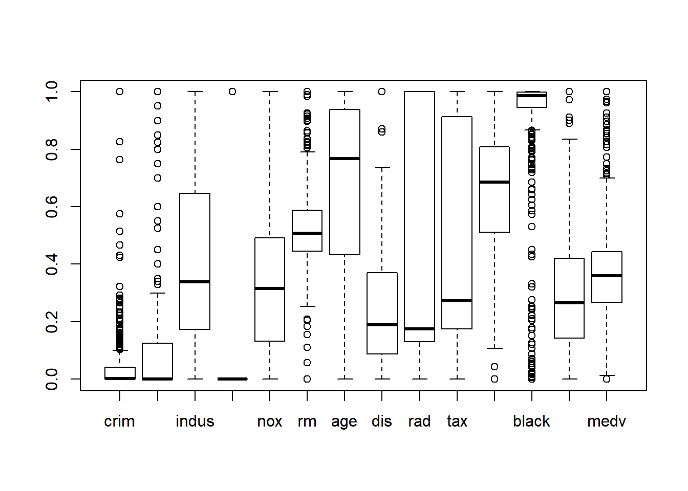
According with the graph above there some som variables with outliers. But the crim predictor variable has the largest number os outliers.
CorBHData<-cor(BHDataScaled)library(corrplot)
## corrplot 0.84 loaded
corrplot(CorBHData, method = "pie",type="lower")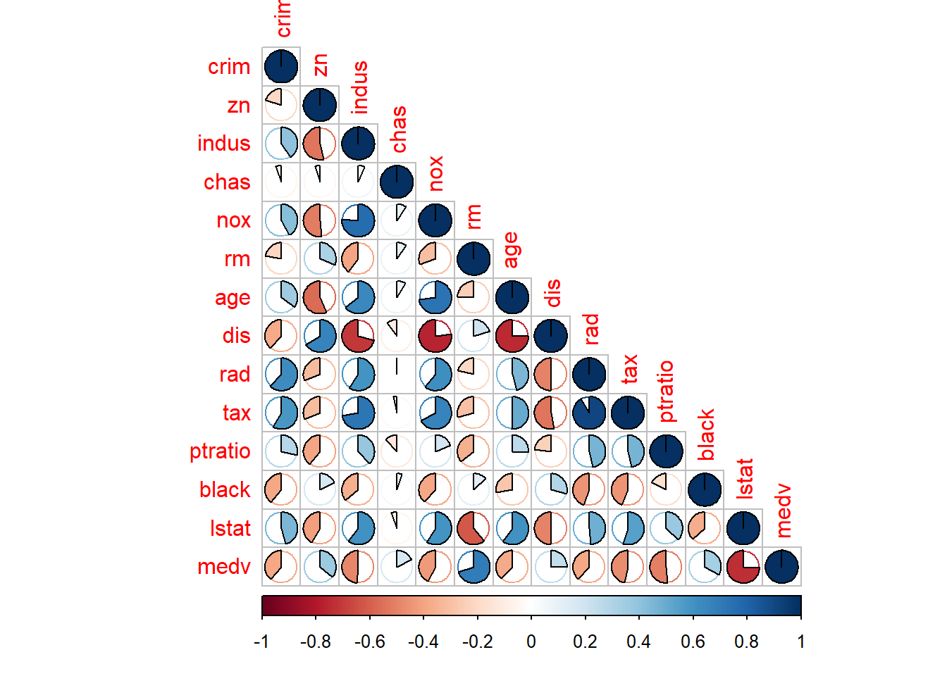
Multiple Linear Model Fitting
LModel1<-lm(medv~.,data=BHDataScaled)summary(LModel1)
##
## Call:
## lm(formula = medv ~ ., data = BHDataScaled)
##
## Residuals:
## Min 1Q Median 3Q Max
## -0.34654 -0.06066 -0.01151 0.03949 0.58221
##
## Coefficients:
## Estimate Std. Error t value Pr(>|t|)
## (Intercept) 0.480450 0.052843 9.092 < 2e-16 ***
## crim -0.213550 0.064978 -3.287 0.001087 **
## zn 0.103157 0.030505 3.382 0.000778 ***
## indus 0.012463 0.037280 0.334 0.738288
## chas 0.059705 0.019146 3.118 0.001925 **
## nox -0.191879 0.041253 -4.651 4.25e-06 ***
## rm 0.441860 0.048470 9.116 < 2e-16 ***
## age 0.001494 0.028504 0.052 0.958229
## dis -0.360592 0.048742 -7.398 6.01e-13 ***
## rad 0.156425 0.033910 4.613 5.07e-06 ***
## tax -0.143629 0.043789 -3.280 0.001112 **
## ptratio -0.199018 0.027328 -7.283 1.31e-12 ***
## black 0.082063 0.023671 3.467 0.000573 ***
## lstat -0.422605 0.040843 -10.347 < 2e-16 ***
## ---
## Signif. codes: 0 '***' 0.001 '**' 0.01 '*' 0.05 '.' 0.1 ' ' 1
##
## Residual standard error: 0.1055 on 492 degrees of freedom
## Multiple R-squared: 0.7406, Adjusted R-squared: 0.7338
## F-statistic: 108.1 on 13 and 492 DF, p-value: < 2.2e-16Pred1 <- predict(LModel1)mse1 <- mean((BHDataScaled$medv - Pred1)^2)mse1
## [1] 0.01081226plot(BHDataScaled[,14],Pred1,
xlab="Actual",ylab="Predicted")
abline(a=0,b=1)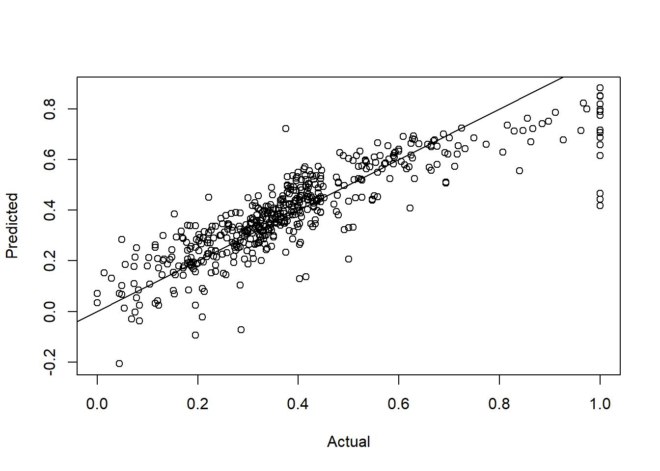
par(mfrow=c(2,2))
plot(LModel1)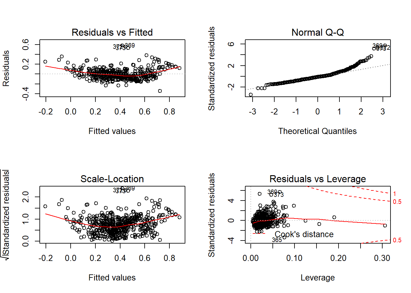
Random Forest Regression Model
library(randomForest)
## randomForest 4.6-14
## Type rfNews() to see new features/changes/bug fixes.
RFModel=randomForest(medv ~ . , data = BHDataScaled)
RFModel
##
## Call:
## randomForest(formula = medv ~ ., data = BHDataScaled)
## Type of random forest: regression
## Number of trees: 500
## No. of variables tried at each split: 4
##
## Mean of squared residuals: 0.00476609
## % Var explained: 88.57summary(RFModel)
## Length Class Mode
## call 3 -none- call
## type 1 -none- character
## predicted 506 -none- numeric
## mse 500 -none- numeric
## rsq 500 -none- numeric
## oob.times 506 -none- numeric
## importance 13 -none- numeric
## importanceSD 0 -none- NULL
## localImportance 0 -none- NULL
## proximity 0 -none- NULL
## ntree 1 -none- numeric
## mtry 1 -none- numeric
## forest 11 -none- list
## coefs 0 -none- NULL
## y 506 -none- numeric
## test 0 -none- NULL
## inbag 0 -none- NULL
## terms 3 terms callplot(RFModel)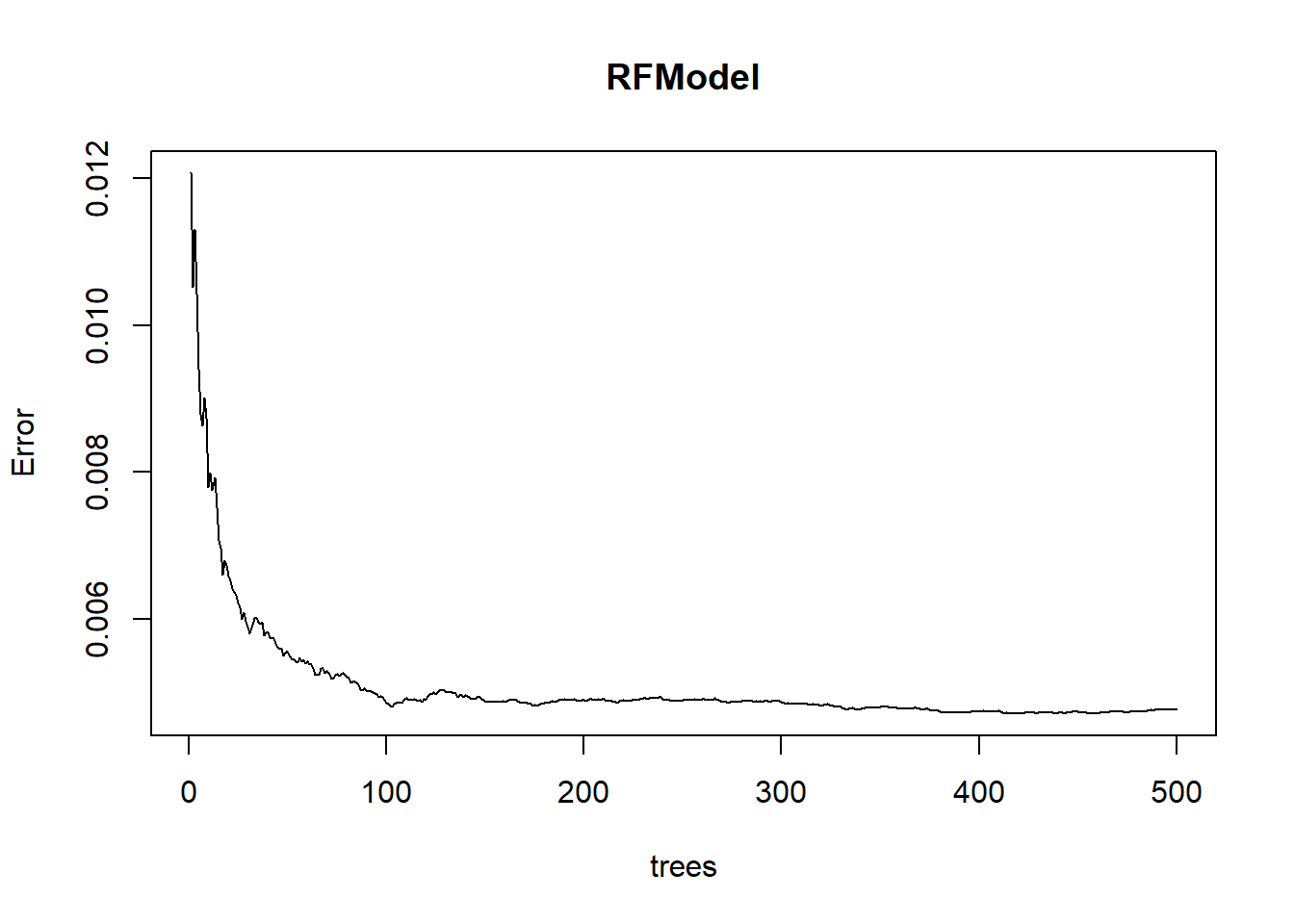
VarImp<-importance(RFModel)
VarImp<-as.matrix(VarImp[order(VarImp[,1], decreasing = TRUE),])
VarImp
##              [,1]
## lstat   6.0574021
## rm      5.7940364
## indus   1.4530514
## nox     1.3531538
## ptratio 1.3171112
## dis     1.2957303
## crim    1.2250947
## tax     0.7204445
## age     0.5578364
## black   0.3748653
## zn      0.1662593
## rad     0.1450710
## chas    0.1365377
varImpPlot(RFModel)
Pred2 <- predict(RFModel)plot(BHDataScaled[,14],Pred2,
xlab="Actual",ylab="Predicted")
abline(a=0,b=1)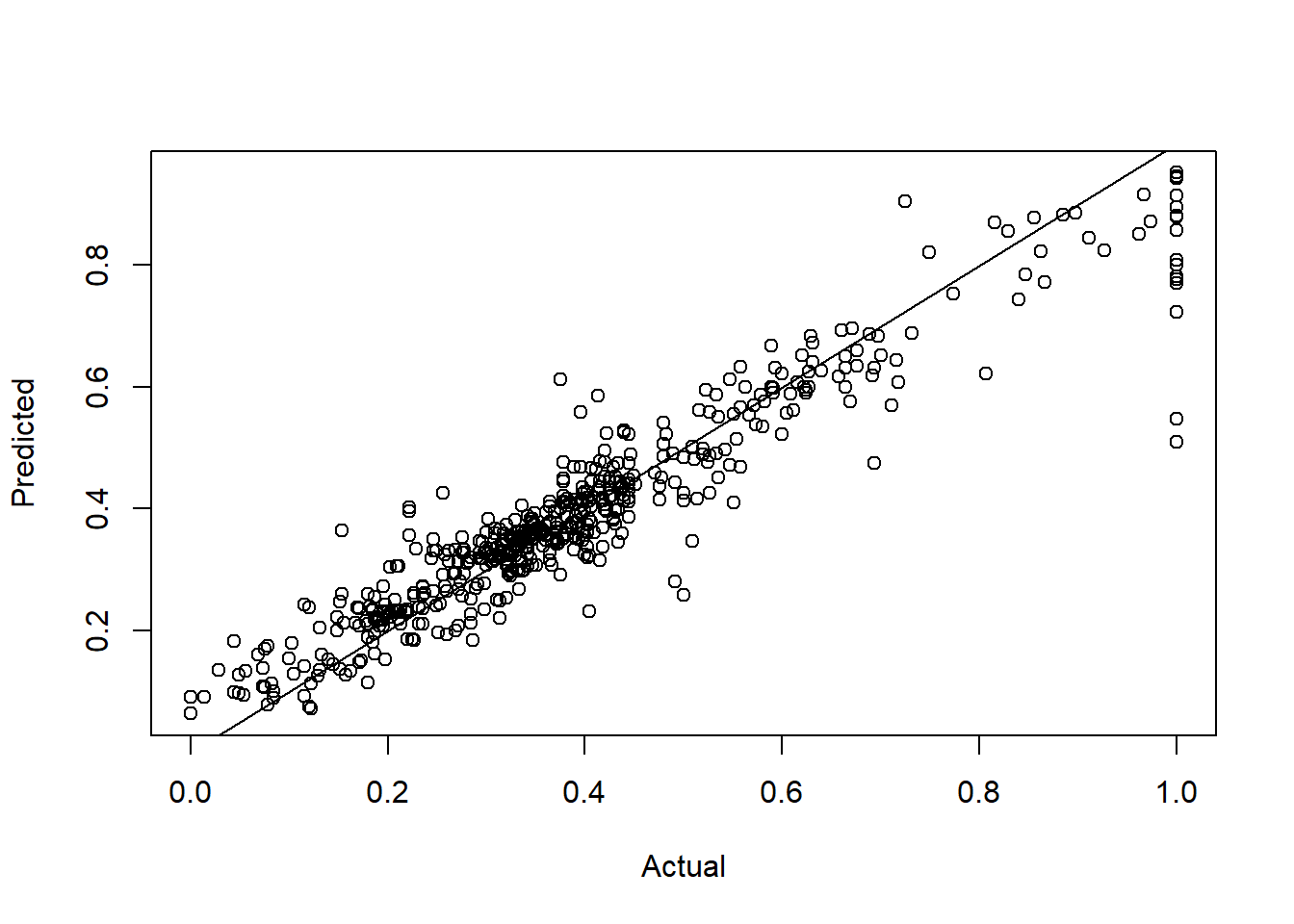
Robust Linear Regression Model
library(MASS)

LModel2 <- rlm(BHDataScaled$medv ~ ., data = BHDataScaled, psi = psi.hampel, init = "lts")
LModel2
## Call:
## rlm(formula = BHDataScaled$medv ~ ., data = BHDataScaled, psi = psi.hampel,
## init = "lts")
## Converged in 10 iterations
##
## Coefficients:
## (Intercept) crim zn indus chas nox
## 0.285874828 -0.192440257 0.069292252 0.003634696 0.029497415 -0.109020365
## rm age dis rad tax ptratio
## 0.680775604 -0.069407410 -0.275014795 0.093236680 -0.145930494 -0.174170551
## black lstat
## 0.095984860 -0.216404818
##
## Degrees of freedom: 506 total; 492 residual
## Scale estimate: 0.0708summary(LModel2)
##
## Call: rlm(formula = BHDataScaled$medv ~ ., data = BHDataScaled, psi = psi.hampel,
## init = "lts")
## Residuals:
## Min 1Q Median 3Q Max
## -0.347670 -0.046918 -0.009419 0.048950 0.767535
##
## Coefficients:
## Value Std. Error t value
## (Intercept) 0.2859 0.0408 7.0063
## crim -0.1924 0.0502 -3.8356
## zn 0.0693 0.0236 2.9418
## indus 0.0036 0.0288 0.1263
## chas 0.0295 0.0148 1.9953
## nox -0.1090 0.0319 -3.4226
## rm 0.6808 0.0374 18.1900
## age -0.0694 0.0220 -3.1536
## dis -0.2750 0.0376 -7.3073
## rad 0.0932 0.0262 3.5609
## tax -0.1459 0.0338 -4.3160
## ptratio -0.1742 0.0211 -8.2540
## black 0.0960 0.0183 5.2515
## lstat -0.2164 0.0315 -6.8621
##
## Residual standard error: 0.07084 on 492 degrees of freedomLM1Coef <- coef(LModel1)
LM2Coef <- coef(LModel2)plot(BHDataScaled$medv, BHDataScaled$lstat)
abline(coef=LM1Coef)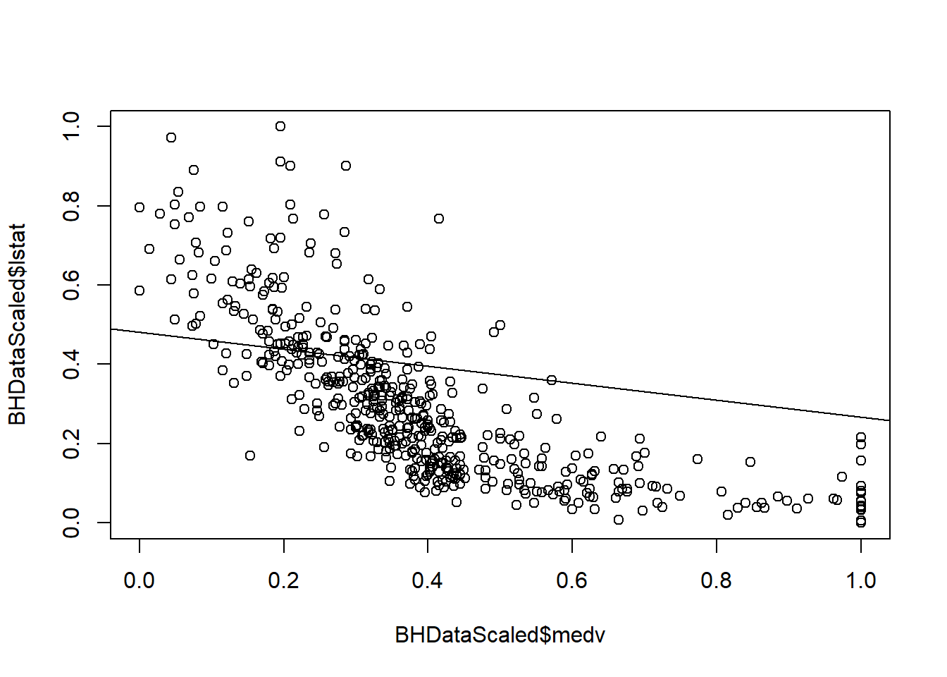
plot(BHDataScaled$medv, BHDataScaled$lstat)
abline(coef=LM2Coef)
boxplot(BHDataScaled$crim)$out
##  [1] 0.1519152 0.1036978 0.1247813 0.2078443 0.2203305 0.1717624 0.1103426
##  [8] 0.2657290 0.2007464 1.0000000 0.1783534 0.1031889 0.2256784 0.1888895
## [15] 0.2741094 0.2539149 0.1610363 0.1300618 0.1500899 0.4309939 0.1113886
## [22] 0.2814411 0.1599404 0.1077824 0.2786941 0.4667072 0.7633424 0.2327741
## [29] 0.1342564 0.1622120 0.5746830 0.1578554 0.2113601 0.3220132 0.5141041
## [36] 0.2031955 0.1217028 0.2914951 0.8264345 0.1326964 0.1245487 0.1353478
## [43] 0.1781949 0.1375845 0.4232396 0.1048958 0.1130268 0.1563122 0.1253692
## [50] 0.1620153 0.1705170 0.1536675 0.1054774 0.2477780 0.1092264 0.1119505
## [57] 0.1438237 0.1198774 0.1114819 0.1047857 0.1068599 0.1749961 0.1468899
## [64] 0.1687884 0.1149454 0.1610363
outliers <- boxplot(BHDataScaled$crim, plot=FALSE)$out
print(outliers)
## [1] 0.1519152 0.1036978 0.1247813 0.2078443 0.2203305 0.1717624 0.1103426
## [8] 0.2657290 0.2007464 1.0000000 0.1783534 0.1031889 0.2256784 0.1888895
## [15] 0.2741094 0.2539149 0.1610363 0.1300618 0.1500899 0.4309939 0.1113886
## [22] 0.2814411 0.1599404 0.1077824 0.2786941 0.4667072 0.7633424 0.2327741
## [29] 0.1342564 0.1622120 0.5746830 0.1578554 0.2113601 0.3220132 0.5141041
## [36] 0.2031955 0.1217028 0.2914951 0.8264345 0.1326964 0.1245487 0.1353478
## [43] 0.1781949 0.1375845 0.4232396 0.1048958 0.1130268 0.1563122 0.1253692
## [50] 0.1620153 0.1705170 0.1536675 0.1054774 0.2477780 0.1092264 0.1119505
## [57] 0.1438237 0.1198774 0.1114819 0.1047857 0.1068599 0.1749961 0.1468899
## [64] 0.1687884 0.1149454 0.1610363BHDataScaled[which(BHDataScaled$crim %in% outliers),]
## crim zn indus chas nox rm age dis rad
## 368 0.1519152 0 0.6466276 0 0.5061728 0.05786549 1.0000000 0.0346461275 1
## 372 0.1036978 0 0.6466276 0 0.5061728 0.50871815 1.0000000 0.0035919214 1
## 374 0.1247813 0 0.6466276 0 0.5823045 0.25771221 1.0000000 0.0040556884 1
## 375 0.2078443 0 0.6466276 0 0.5823045 0.11055758 1.0000000 0.0006729169 1
## 376 0.2203305 0 0.6466276 0 0.5884774 0.71891167 0.9783728 0.0169775118 1
## 377 0.1717624 0 0.6466276 0 0.5884774 0.59168423 0.9309990 0.0195782448 1
## 378 0.1103426 0 0.6466276 0 0.5884774 0.61946733 0.9876416 0.0207694896 1
## 379 0.2657290 0 0.6466276 0 0.5884774 0.54014179 0.9608651 0.0233247552 1
## 380 0.2007464 0 0.6466276 0 0.5884774 0.51005940 1.0000000 0.0233247552 1
## 381 1.0000000 0 0.6466276 0 0.5884774 0.65280705 0.9165808 0.0260891706 1
## 382 0.1783534 0 0.6466276 0 0.5884774 0.57175704 0.9907312 0.0354281661 1
## 383 0.1031889 0 0.6466276 0 0.6481481 0.37842499 1.0000000 0.0409933709 1
## 385 0.2256784 0 0.6466276 0 0.6481481 0.15462732 0.9093718 0.0281806691 1
## 386 0.1888895 0 0.6466276 0 0.6481481 0.32879862 0.9804325 0.0269621439 1
## 387 0.2741094 0 0.6466276 0 0.6481481 0.20904388 1.0000000 0.0306995608 1
## 388 0.2539149 0 0.6466276 0 0.6481481 0.27572332 0.8918641 0.0353554183 1
## 389 0.1610363 0 0.6466276 0 0.6481481 0.25273041 1.0000000 0.0418208768 1
## 393 0.1300618 0 0.6466276 0 0.6481481 0.28262119 0.9691040 0.0582345934 1
## 395 0.1500899 0 0.6466276 0 0.6337449 0.44567925 0.9454171 0.0593349035 1
## 399 0.4309939 0 0.6466276 0 0.6337449 0.36252156 1.0000000 0.0327364985 1
## 400 0.1113886 0 0.6466276 0 0.6337449 0.43897298 0.7713697 0.0337185934 1
## 401 0.2814411 0 0.6466276 0 0.6337449 0.46484001 1.0000000 0.0417572225 1
## 402 0.1599404 0 0.6466276 0 0.6337449 0.53305231 1.0000000 0.0404204821 1
## 403 0.1077824 0 0.6466276 0 0.6337449 0.54474037 1.0000000 0.0463221453 1
## 404 0.2786941 0 0.6466276 0 0.6337449 0.34259437 0.9588054 0.0521237803 1
## 405 0.4667072 0 0.6466276 0 0.6337449 0.37746695 0.8496395 0.0434486082 1
## 406 0.7633424 0 0.6466276 0 0.6337449 0.40659130 1.0000000 0.0268984896 1
## 407 0.2327741 0 0.6466276 0 0.5637860 0.11055758 1.0000000 0.0044103338 1
## 408 0.1342564 0 0.6466276 0 0.5637860 0.39222073 1.0000000 0.0141494421 1
## 410 0.1622120 0 0.6466276 0 0.4362140 0.63058057 1.0000000 0.0305449718 1
## 411 0.5746830 0 0.6466276 0 0.4362140 0.42077026 1.0000000 0.0257708991 1
## 412 0.1578554 0 0.6466276 0 0.4362140 0.59321709 1.0000000 0.0361829243 1
## 413 0.2113601 0 0.6466276 0 0.4362140 0.20444530 1.0000000 0.0385836008 1
## 414 0.3220132 0 0.6466276 0 0.4362140 0.30542249 1.0000000 0.0418117833 1
## 415 0.5141041 0 0.6466276 0 0.6337449 0.18356007 1.0000000 0.0480680919 1
## 416 0.2031955 0 0.6466276 0 0.6049383 0.55048860 1.0000000 0.0641180696 1
## 417 0.1217028 0 0.6466276 0 0.6049383 0.61716804 0.9052523 0.0627358619 1
## 418 0.2914951 0 0.6466276 0 0.6049383 0.33397203 0.8877446 0.0470950904 1
## 419 0.8264345 0 0.6466276 0 0.6049383 0.45909178 1.0000000 0.0611990652 1
## 420 0.1326964 0 0.6466276 0 0.6851852 0.62521556 0.7579815 0.0604170266 1
## 421 0.1245487 0 0.6466276 0 0.6851852 0.54608162 1.0000000 0.0663186898 1
## 423 0.1353478 0 0.6466276 0 0.4711934 0.39988504 0.8722966 0.0747119643 1
## 426 0.1781949 0 0.6466276 0 0.6049383 0.44740372 0.9526262 0.0709290800 1
## 427 0.1375845 0 0.6466276 0 0.4094650 0.43609887 0.5849640 0.0789313352 1
## 428 0.4232396 0 0.6466276 0 0.6049383 0.50603564 0.7806385 0.0666824287 1
## 430 0.1048958 0 0.6466276 0 0.6049383 0.54014179 0.9546859 0.0762578545 1
## 432 0.1130268 0 0.6466276 0 0.4094650 0.62694003 0.9412976 0.0871700206 1
## 435 0.1563122 0 0.6466276 0 0.6748971 0.50718528 0.9485067 0.0993552728 1
## 436 0.1253692 0 0.6466276 0 0.7304527 0.58785208 0.9443872 0.0904891378 1
## 437 0.1620153 0 0.6466276 0 0.7304527 0.55566200 0.9309990 0.0793860088 1
## 438 0.1705170 0 0.6466276 0 0.7304527 0.49645526 1.0000000 0.0713473797 1
## 439 0.1536675 0 0.6466276 0 0.7304527 0.45487641 0.8753862 0.0628358901 1
## 440 0.1054774 0 0.6466276 0 0.7304527 0.39586128 0.9371782 0.0625267121 1
## 441 0.2477780 0 0.6466276 0 0.7304527 0.43245833 0.9217302 0.0669825133 1
## 442 0.1092264 0 0.6466276 0 0.7304527 0.54512359 0.9711637 0.0850694287 1
## 444 0.1119505 0 0.6466276 0 0.7304527 0.56026059 1.0000000 0.0771853886 1
## 445 0.1438237 0 0.6466276 0 0.7304527 0.43935620 0.9649846 0.0696559940 1
## 446 0.1198774 0 0.6466276 0 0.7304527 0.55527879 0.9464470 0.0780492684 1
## 448 0.1114819 0 0.6466276 0 0.7304527 0.51542441 0.9649846 0.0971546527 1
## 449 0.1047857 0 0.6466276 0 0.6748971 0.50277831 0.9866117 0.1029381007 1
## 455 0.1068599 0 0.6466276 0 0.6748971 0.60682123 0.9392379 0.1242622921 1
## 469 0.1749961 0 0.6466276 0 0.4012346 0.45315194 0.7013388 0.1617546763 1
## 470 0.1468899 0 0.6466276 0 0.4012346 0.41233953 0.5540680 0.1540525057 1
## 478 0.1687884 0 0.6466276 0 0.4711934 0.33397203 0.9721936 0.0883067046 1
## 479 0.1149454 0 0.6466276 0 0.4711934 0.50277831 0.9660144 0.0946539479 1
## 480 0.1610363 0 0.6466276 0 0.4711934 0.51120904 0.8764161 0.0747119643 1
## tax ptratio black lstat medv
## 368 0.9141221 0.8085106 0.330576428 0.3200883 0.40222222
## 372 0.9141221 0.8085106 0.922462051 0.2152318 1.00000000
## 374 0.9141221 0.8085106 1.000000000 0.9116998 0.19555556
## 375 0.9141221 0.8085106 1.000000000 1.0000000 0.19555556
## 376 0.9141221 0.8085106 1.000000000 0.3231236 0.22222222
## 377 0.9141221 0.8085106 0.914569570 0.5935430 0.19777778
## 378 0.9141221 0.8085106 1.000000000 0.5383554 0.18444444
## 379 0.9141221 0.8085106 1.000000000 0.6059603 0.18000000
## 380 0.9141221 0.8085106 0.992031873 0.5532561 0.11555556
## 381 0.9141221 0.8085106 1.000000000 0.4271523 0.12000000
## 382 0.9141221 0.8085106 1.000000000 0.5339404 0.13111111
## 383 0.9141221 0.8085106 1.000000000 0.6034768 0.14000000
## 385 0.9141221 0.8085106 0.719930405 0.7974614 0.08444444
## 386 0.9141221 0.8085106 1.000000000 0.8024283 0.04888889
## 387 0.9141221 0.8085106 1.000000000 0.7326159 0.12222222
## 388 0.9141221 0.8085106 1.000000000 0.8349890 0.05333333
## 389 0.9141221 0.8085106 0.939533007 0.7971854 0.11555556
## 393 0.9141221 0.8085106 1.000000000 0.6608720 0.10444444
## 395 0.9141221 0.8085106 1.000000000 0.4034216 0.17111111
## 399 0.9141221 0.8085106 1.000000000 0.7963576 0.00000000
## 400 0.9141221 0.8085106 0.851883605 0.7792494 0.02888889
## 401 0.9141221 0.8085106 1.000000000 0.6909492 0.01333333
## 402 0.9141221 0.8085106 1.000000000 0.5129691 0.04888889
## 403 0.9141221 0.8085106 0.947576781 0.5126932 0.15777778
## 404 0.9141221 0.8085106 1.000000000 0.4977925 0.07333333
## 405 0.9141221 0.8085106 0.829946039 0.7077815 0.07777778
## 406 0.9141221 0.8085106 0.969917797 0.5863687 0.00000000
## 407 0.9141221 0.8085106 0.932724797 0.5963024 0.15333333
## 408 0.9141221 0.8085106 0.836577740 0.2869757 0.50888889
## 410 0.9141221 0.8085106 0.451459983 0.4980684 0.50000000
## 411 0.9141221 0.8085106 0.005749155 0.2312362 0.22222222
## 412 0.9141221 0.8085106 0.087573756 0.5378035 0.27111111
## 413 0.9141221 0.8085106 0.071788794 0.9006623 0.28666667
## 414 0.9141221 0.8085106 0.531166473 0.5063466 0.25111111
## 415 0.9141221 0.8085106 0.221771143 0.9726821 0.04444444
## 416 0.9141221 0.8085106 0.067905593 0.7538631 0.04888889
## 417 0.9141221 0.8085106 0.053583136 0.6639073 0.05555556
## 418 0.9141221 0.8085106 0.320338898 0.6873620 0.12000000
## 419 0.9141221 0.8085106 0.040672752 0.5212472 0.08444444
## 420 0.9141221 0.8085106 0.121362651 0.5797461 0.07555556
## 421 0.9141221 0.8085106 0.802940138 0.3667219 0.26000000
## 423 0.9141221 0.8085106 0.734353724 0.3413355 0.35111111
## 426 0.9141221 0.8085106 0.018558677 0.6252759 0.07333333
## 427 0.9141221 0.8085106 0.061349539 0.3852097 0.11555556
## 428 0.9141221 0.8085106 0.046648848 0.3529249 0.13111111
## 430 0.9141221 0.8085106 0.152302184 0.6167219 0.10000000
## 432 0.9141221 0.8085106 0.204271522 0.4955850 0.20222222
## 435 0.9141221 0.8085106 0.252937617 0.3708609 0.14888889
## 436 0.9141221 0.8085106 0.276186394 0.5943709 0.18666667
## 437 0.9141221 0.8085106 0.068510767 0.4503311 0.10222222
## 438 0.9141221 0.8085106 0.022694034 0.6821192 0.08222222
## 439 0.9141221 0.8085106 0.173054617 0.8910044 0.07555556
## 440 0.9141221 0.8085106 1.000000000 0.5836093 0.17333333
## 441 0.9141221 0.8085106 0.986257502 0.5623620 0.12222222
## 442 0.9141221 0.8085106 0.972414141 0.4908940 0.26888889
## 444 0.9141221 0.8085106 0.974355742 0.4724062 0.23111111
## 445 0.9141221 0.8085106 0.605678552 0.6087196 0.12888889
## 446 0.9141221 0.8085106 0.107771446 0.6139625 0.15111111
## 448 0.9141221 0.8085106 0.978869333 0.4059051 0.16888889
## 449 0.9141221 0.8085106 1.000000000 0.4525386 0.20222222
## 455 0.9141221 0.8085106 0.016037117 0.4685430 0.22000000
## 469 0.9141221 0.8085106 0.928992889 0.4525386 0.31333333
## 470 0.9141221 0.8085106 1.000000000 0.3595475 0.33555556
## 478 0.9141221 0.8085106 0.880427656 0.6396247 0.15555556
## 479 0.9141221 0.8085106 0.956629179 0.4497792 0.21333333
## 480 0.9141221 0.8085106 0.965757224 0.3140177 0.36444444boxplot(BHDataScaled$crim)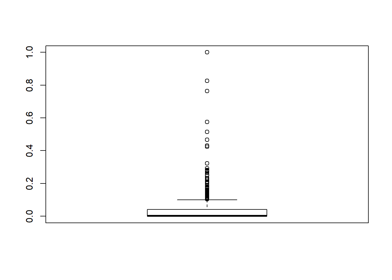
remove_outliers <- function(x, na.rm = TRUE, ...) {
  qnt <- quantile(x, probs=c(.25, .75), na.rm = na.rm, ...)
  H <- 1.5 * IQR(x, na.rm = na.rm)
  y <- x
  y[x < (qnt[1] - H)] <- NA
  y[x > (qnt[2] + H)] <- NA
  y
}
remove_outliers(BHDataScaled$crim)
## [1] 0.000000e+00 2.359225e-04 2.356977e-04 2.927957e-04 7.050701e-04
## [6] 2.644715e-04 9.213230e-04 1.553672e-03 2.303251e-03 1.840173e-03
## [11] 2.456674e-03 1.249299e-03 9.830293e-04 7.007315e-03 7.099481e-03
## [16] 6.980677e-03 1.177488e-02 8.743184e-03 8.951232e-03 8.086782e-03
## [21] 1.399878e-02 9.505689e-03 1.378163e-02 1.103868e-02 8.361706e-03
## [26] 9.376432e-03 7.481071e-03 1.067159e-02 8.617186e-03 1.119626e-02
## [31] 1.263900e-02 1.515569e-02 1.552964e-02 1.287402e-02 1.805667e-02
## [36] 6.502201e-04 1.024167e-03 8.297190e-04 1.896485e-03 2.395193e-04
## [41] 3.065082e-04 1.361360e-03 1.519391e-03 1.720133e-03 1.307971e-03
## [46] 1.855684e-03 2.046086e-03 2.505904e-03 2.782402e-03 2.399127e-03
## [51] 9.262685e-04 4.164331e-04 5.314158e-04 4.888171e-04 8.182544e-05
## [56] 7.631796e-05 1.599418e-04 8.991807e-05 1.664945e-03 1.089807e-03
## [61] 1.607286e-03 1.858944e-03 1.168373e-03 1.350794e-03 1.482524e-04
## [66] 3.317977e-04 4.211538e-04 5.796344e-04 1.452402e-03 1.369452e-03
## [71] 9.209858e-04 1.713389e-03 9.589762e-04 2.125101e-03 8.164561e-04
## [76] 9.980906e-04 1.070137e-03 9.076105e-04 5.635615e-04 8.716433e-04
## [81] 3.912560e-04 4.304828e-04 3.402275e-04 3.280886e-04 4.975841e-04
## [86] 5.735649e-04 5.120834e-04 7.327199e-04 5.651351e-04 5.248967e-04
## [91] 4.554350e-04 3.709120e-04 4.013718e-04 2.521078e-04 4.116000e-04
## [96] 1.300665e-03 1.221987e-03 1.287065e-03 8.491638e-04 7.000122e-04
## [101] 1.599867e-03 1.213894e-03 2.500172e-03 2.307410e-03 1.498035e-03
## [106] 1.419582e-03 1.853211e-03 1.403284e-03 1.367879e-03 2.892102e-03
## [111] 1.142072e-03 1.062382e-03 1.314715e-03 2.425540e-03 1.528495e-03
## [116] 1.854785e-03 1.407892e-03 1.625944e-03 1.396652e-03 1.556032e-03
## [121] 7.043957e-04 7.342934e-04 9.741499e-04 1.619200e-03 1.035969e-03
## [126] 1.828709e-03 4.282685e-03 2.841748e-03 3.586719e-03 9.834002e-03
## [131] 3.751157e-03 1.333732e-02 6.560984e-03 3.636062e-03 1.090088e-02
## [136] 6.198277e-03 3.555361e-03 3.889069e-03 2.736656e-03 6.049238e-03
## [141] 3.198611e-03 1.823449e-02 3.725677e-02 4.598275e-02 3.117257e-02
## [146] 2.667217e-02 2.415121e-02 2.655168e-02 2.612873e-02 3.065813e-02
## [151] 1.854875e-02 1.674724e-02 1.259145e-02 2.408523e-02 1.582030e-02
## [156] 3.966162e-02 2.742906e-02 1.368171e-02 1.502216e-02 1.594585e-02
## [161] 1.424235e-02 1.637678e-02 2.054010e-02 1.700238e-02 2.513255e-02
## [166] 3.279402e-02 2.252302e-02 2.016368e-02 2.578491e-02 2.746109e-02
## [171] 1.350007e-02 2.593664e-02 1.492865e-03 9.605498e-04 8.783872e-04
## [176] 6.779823e-04 7.182206e-04 5.387216e-04 6.755095e-04 5.786228e-04
## [181] 6.694400e-04 7.031593e-04 9.521200e-04 1.053840e-03 8.627639e-04
## [186] 6.086329e-04 5.586160e-04 8.140957e-04 1.342814e-03 8.697325e-04
## [191] 9.481861e-04 7.057445e-04 9.027774e-04 1.747783e-04 9.070485e-05
## [196] 8.418579e-05 3.797915e-04 4.534119e-04 3.524788e-04 2.830171e-04
## [201] 1.288076e-04 3.161744e-04 1.736543e-04 3.234803e-04 1.547715e-04
## [206] 1.462293e-03 2.510625e-03 2.761272e-03 1.456111e-03 4.826240e-03
## [211] 1.889853e-03 4.152641e-03 2.370128e-03 1.508376e-03 3.183437e-03
## [216] 2.154662e-03 4.414977e-04 7.172090e-04 1.173094e-03 1.213107e-03
## [221] 3.953810e-03 4.511527e-03 6.937629e-03 6.838045e-03 3.473198e-03
## [226] 5.851531e-03 4.224126e-03 4.564016e-03 3.280548e-03 4.894465e-03
## [231] 5.964715e-03 5.132524e-03 6.395086e-03 3.654608e-03 4.963365e-03
## [236] 3.643143e-03 5.780158e-03 5.681811e-03 8.555704e-04 9.688672e-04
## [241] 1.202317e-03 1.121728e-03 1.085536e-03 1.362821e-03 2.245254e-03
## [246] 2.079468e-03 3.748572e-03 2.138364e-03 1.776669e-03 2.072724e-03
## [251] 1.505903e-03 2.335285e-03 8.529853e-04 4.075761e-03 4.706087e-04
## [256] 3.277514e-04 1.018322e-04 6.802527e-03 7.386657e-03 7.309552e-03
## [261] 5.999671e-03 5.932345e-03 5.775213e-03 9.204688e-03 6.111619e-03
## [266] 8.489390e-03 8.760043e-03 6.429367e-03 6.004054e-03 9.478489e-04
## [271] 3.291451e-03 1.751042e-03 1.217041e-03 2.422842e-03 5.633367e-04
## [276] 1.008431e-03 1.105655e-03 6.176248e-04 8.256727e-04 2.293585e-03
## [281] 3.311233e-04 3.453978e-04 6.178495e-04 9.767350e-05 3.079694e-05
## [286] 5.215248e-05 1.498260e-04 3.640558e-04 4.448697e-04 4.119372e-04
## [291] 3.225811e-04 8.153321e-04 3.352820e-04 8.579308e-04 8.505126e-04
## [296] 1.382490e-03 5.327646e-04 1.514108e-03 6.557275e-04 5.540077e-04
## [301] 4.254249e-04 3.265150e-04 9.704408e-04 1.052941e-03 5.488374e-04
## [306] 5.447911e-04 7.722838e-04 4.833096e-04 5.469941e-03 3.856136e-03
## [311] 2.955112e-02 8.812983e-03 2.870297e-03 2.956731e-03 4.078684e-03
## [316] 2.778918e-03 3.506243e-03 2.685178e-03 4.447573e-03 5.273133e-03
## [321] 1.812748e-03 1.969993e-03 3.875694e-03 3.120157e-03 3.762734e-03
## [326] 2.085425e-03 3.339894e-03 2.638084e-03 6.726996e-04 6.847261e-04
## [331] 4.396994e-04 4.935378e-04 3.185348e-04 5.002817e-04 3.491069e-04
## [336] 3.741716e-04 3.141513e-04 2.707658e-04 3.005512e-04 5.468143e-04
## [341] 6.203223e-04 7.519399e-05 2.097339e-04 2.147918e-04 2.716650e-04
## [346] 2.788584e-04 6.215587e-04 1.391482e-04 9.767350e-05 2.548053e-04
## [351] 6.270661e-04 8.225256e-04 7.431729e-04 1.210522e-04 4.123868e-04
## [356] 1.127011e-03 1.008953e-01 4.319866e-02 5.839561e-02 4.782506e-02
## [361] 5.097905e-02 4.305412e-02 4.127127e-02 4.738761e-02 3.897903e-02
## [366] 5.113585e-02 4.148179e-02 NA 5.498378e-02 6.365817e-02
## [371] 7.342305e-02 NA 9.285086e-02 NA NA
## [376] NA NA NA NA NA
## [381] NA NA NA 8.976251e-02 NA
## [386] NA NA NA NA 9.155256e-02
## [391] 7.818185e-02 5.942157e-02 NA 9.709398e-02 NA
## [396] 9.790313e-02 6.592939e-02 8.616062e-02 NA NA
## [401] NA NA NA NA NA
## [406] NA NA NA 8.314690e-02 NA
## [411] NA NA NA NA NA
## [416] NA NA NA NA NA
## [421] NA 7.886118e-02 NA 7.917399e-02 9.875027e-02
## [426] NA NA NA 8.273350e-02 NA
## [431] 9.537846e-02 NA 7.235853e-02 6.265885e-02 NA
## [436] NA NA NA NA NA
## [441] NA NA 6.361760e-02 NA NA
## [446] NA 7.060536e-02 NA NA 8.451950e-02
## [451] 7.543452e-02 6.108607e-02 5.714125e-02 9.263551e-02 NA
## [456] 5.334446e-02 5.240549e-02 9.210151e-02 8.706216e-02 7.637248e-02
## [461] 5.401615e-02 4.143863e-02 7.472866e-02 6.535729e-02 8.804103e-02
## [466] 3.548707e-02 4.235883e-02 4.963433e-02 NA NA
## [471] 4.880832e-02 4.531972e-02 4.004007e-02 5.215889e-02 9.047410e-02
## [476] 7.178609e-02 5.468244e-02 NA NA NA
## [481] 6.538943e-02 6.408753e-02 6.434582e-02 3.160688e-02 2.666352e-02
## [486] 4.122013e-02 6.390286e-02 5.428073e-02 1.624595e-03 1.989999e-03
## [491] 2.260765e-03 1.117457e-03 1.180175e-03 1.876927e-03 3.071264e-03
## [496] 1.940769e-03 3.183999e-03 2.945491e-03 2.616616e-03 1.927731e-03
## [501] 2.450942e-03 6.329108e-04 4.377886e-04 6.118925e-04 1.160730e-03
## [506] 4.618417e-04BHDataScaled$crim[!BHDataScaled$crim %in% boxplot.stats(BHDataScaled$crim)$out]
## [1] 0.000000e+00 2.359225e-04 2.356977e-04 2.927957e-04 7.050701e-04
## [6] 2.644715e-04 9.213230e-04 1.553672e-03 2.303251e-03 1.840173e-03
## [11] 2.456674e-03 1.249299e-03 9.830293e-04 7.007315e-03 7.099481e-03
## [16] 6.980677e-03 1.177488e-02 8.743184e-03 8.951232e-03 8.086782e-03
## [21] 1.399878e-02 9.505689e-03 1.378163e-02 1.103868e-02 8.361706e-03
## [26] 9.376432e-03 7.481071e-03 1.067159e-02 8.617186e-03 1.119626e-02
## [31] 1.263900e-02 1.515569e-02 1.552964e-02 1.287402e-02 1.805667e-02
## [36] 6.502201e-04 1.024167e-03 8.297190e-04 1.896485e-03 2.395193e-04
## [41] 3.065082e-04 1.361360e-03 1.519391e-03 1.720133e-03 1.307971e-03
## [46] 1.855684e-03 2.046086e-03 2.505904e-03 2.782402e-03 2.399127e-03
## [51] 9.262685e-04 4.164331e-04 5.314158e-04 4.888171e-04 8.182544e-05
## [56] 7.631796e-05 1.599418e-04 8.991807e-05 1.664945e-03 1.089807e-03
## [61] 1.607286e-03 1.858944e-03 1.168373e-03 1.350794e-03 1.482524e-04
## [66] 3.317977e-04 4.211538e-04 5.796344e-04 1.452402e-03 1.369452e-03
## [71] 9.209858e-04 1.713389e-03 9.589762e-04 2.125101e-03 8.164561e-04
## [76] 9.980906e-04 1.070137e-03 9.076105e-04 5.635615e-04 8.716433e-04
## [81] 3.912560e-04 4.304828e-04 3.402275e-04 3.280886e-04 4.975841e-04
## [86] 5.735649e-04 5.120834e-04 7.327199e-04 5.651351e-04 5.248967e-04
## [91] 4.554350e-04 3.709120e-04 4.013718e-04 2.521078e-04 4.116000e-04
## [96] 1.300665e-03 1.221987e-03 1.287065e-03 8.491638e-04 7.000122e-04
## [101] 1.599867e-03 1.213894e-03 2.500172e-03 2.307410e-03 1.498035e-03
## [106] 1.419582e-03 1.853211e-03 1.403284e-03 1.367879e-03 2.892102e-03
## [111] 1.142072e-03 1.062382e-03 1.314715e-03 2.425540e-03 1.528495e-03
## [116] 1.854785e-03 1.407892e-03 1.625944e-03 1.396652e-03 1.556032e-03
## [121] 7.043957e-04 7.342934e-04 9.741499e-04 1.619200e-03 1.035969e-03
## [126] 1.828709e-03 4.282685e-03 2.841748e-03 3.586719e-03 9.834002e-03
## [131] 3.751157e-03 1.333732e-02 6.560984e-03 3.636062e-03 1.090088e-02
## [136] 6.198277e-03 3.555361e-03 3.889069e-03 2.736656e-03 6.049238e-03
## [141] 3.198611e-03 1.823449e-02 3.725677e-02 4.598275e-02 3.117257e-02
## [146] 2.667217e-02 2.415121e-02 2.655168e-02 2.612873e-02 3.065813e-02
## [151] 1.854875e-02 1.674724e-02 1.259145e-02 2.408523e-02 1.582030e-02
## [156] 3.966162e-02 2.742906e-02 1.368171e-02 1.502216e-02 1.594585e-02
## [161] 1.424235e-02 1.637678e-02 2.054010e-02 1.700238e-02 2.513255e-02
## [166] 3.279402e-02 2.252302e-02 2.016368e-02 2.578491e-02 2.746109e-02
## [171] 1.350007e-02 2.593664e-02 1.492865e-03 9.605498e-04 8.783872e-04
## [176] 6.779823e-04 7.182206e-04 5.387216e-04 6.755095e-04 5.786228e-04
## [181] 6.694400e-04 7.031593e-04 9.521200e-04 1.053840e-03 8.627639e-04
## [186] 6.086329e-04 5.586160e-04 8.140957e-04 1.342814e-03 8.697325e-04
## [191] 9.481861e-04 7.057445e-04 9.027774e-04 1.747783e-04 9.070485e-05
## [196] 8.418579e-05 3.797915e-04 4.534119e-04 3.524788e-04 2.830171e-04
## [201] 1.288076e-04 3.161744e-04 1.736543e-04 3.234803e-04 1.547715e-04
## [206] 1.462293e-03 2.510625e-03 2.761272e-03 1.456111e-03 4.826240e-03
## [211] 1.889853e-03 4.152641e-03 2.370128e-03 1.508376e-03 3.183437e-03
## [216] 2.154662e-03 4.414977e-04 7.172090e-04 1.173094e-03 1.213107e-03
## [221] 3.953810e-03 4.511527e-03 6.937629e-03 6.838045e-03 3.473198e-03
## [226] 5.851531e-03 4.224126e-03 4.564016e-03 3.280548e-03 4.894465e-03
## [231] 5.964715e-03 5.132524e-03 6.395086e-03 3.654608e-03 4.963365e-03
## [236] 3.643143e-03 5.780158e-03 5.681811e-03 8.555704e-04 9.688672e-04
## [241] 1.202317e-03 1.121728e-03 1.085536e-03 1.362821e-03 2.245254e-03
## [246] 2.079468e-03 3.748572e-03 2.138364e-03 1.776669e-03 2.072724e-03
## [251] 1.505903e-03 2.335285e-03 8.529853e-04 4.075761e-03 4.706087e-04
## [256] 3.277514e-04 1.018322e-04 6.802527e-03 7.386657e-03 7.309552e-03
## [261] 5.999671e-03 5.932345e-03 5.775213e-03 9.204688e-03 6.111619e-03
## [266] 8.489390e-03 8.760043e-03 6.429367e-03 6.004054e-03 9.478489e-04
## [271] 3.291451e-03 1.751042e-03 1.217041e-03 2.422842e-03 5.633367e-04
## [276] 1.008431e-03 1.105655e-03 6.176248e-04 8.256727e-04 2.293585e-03
## [281] 3.311233e-04 3.453978e-04 6.178495e-04 9.767350e-05 3.079694e-05
## [286] 5.215248e-05 1.498260e-04 3.640558e-04 4.448697e-04 4.119372e-04
## [291] 3.225811e-04 8.153321e-04 3.352820e-04 8.579308e-04 8.505126e-04
## [296] 1.382490e-03 5.327646e-04 1.514108e-03 6.557275e-04 5.540077e-04
## [301] 4.254249e-04 3.265150e-04 9.704408e-04 1.052941e-03 5.488374e-04
## [306] 5.447911e-04 7.722838e-04 4.833096e-04 5.469941e-03 3.856136e-03
## [311] 2.955112e-02 8.812983e-03 2.870297e-03 2.956731e-03 4.078684e-03
## [316] 2.778918e-03 3.506243e-03 2.685178e-03 4.447573e-03 5.273133e-03
## [321] 1.812748e-03 1.969993e-03 3.875694e-03 3.120157e-03 3.762734e-03
## [326] 2.085425e-03 3.339894e-03 2.638084e-03 6.726996e-04 6.847261e-04
## [331] 4.396994e-04 4.935378e-04 3.185348e-04 5.002817e-04 3.491069e-04
## [336] 3.741716e-04 3.141513e-04 2.707658e-04 3.005512e-04 5.468143e-04
## [341] 6.203223e-04 7.519399e-05 2.097339e-04 2.147918e-04 2.716650e-04
## [346] 2.788584e-04 6.215587e-04 1.391482e-04 9.767350e-05 2.548053e-04
## [351] 6.270661e-04 8.225256e-04 7.431729e-04 1.210522e-04 4.123868e-04
## [356] 1.127011e-03 1.008953e-01 4.319866e-02 5.839561e-02 4.782506e-02
## [361] 5.097905e-02 4.305412e-02 4.127127e-02 4.738761e-02 3.897903e-02
## [366] 5.113585e-02 4.148179e-02 5.498378e-02 6.365817e-02 7.342305e-02
## [371] 9.285086e-02 8.976251e-02 9.155256e-02 7.818185e-02 5.942157e-02
## [376] 9.709398e-02 9.790313e-02 6.592939e-02 8.616062e-02 8.314690e-02
## [381] 7.886118e-02 7.917399e-02 9.875027e-02 8.273350e-02 9.537846e-02
## [386] 7.235853e-02 6.265885e-02 6.361760e-02 7.060536e-02 8.451950e-02
## [391] 7.543452e-02 6.108607e-02 5.714125e-02 9.263551e-02 5.334446e-02
## [396] 5.240549e-02 9.210151e-02 8.706216e-02 7.637248e-02 5.401615e-02
## [401] 4.143863e-02 7.472866e-02 6.535729e-02 8.804103e-02 3.548707e-02
## [406] 4.235883e-02 4.963433e-02 4.880832e-02 4.531972e-02 4.004007e-02
## [411] 5.215889e-02 9.047410e-02 7.178609e-02 5.468244e-02 6.538943e-02
## [416] 6.408753e-02 6.434582e-02 3.160688e-02 2.666352e-02 4.122013e-02
## [421] 6.390286e-02 5.428073e-02 1.624595e-03 1.989999e-03 2.260765e-03
## [426] 1.117457e-03 1.180175e-03 1.876927e-03 3.071264e-03 1.940769e-03
## [431] 3.183999e-03 2.945491e-03 2.616616e-03 1.927731e-03 2.450942e-03
## [436] 6.329108e-04 4.377886e-04 6.118925e-04 1.160730e-03 4.618417e-04Car Dataset
# Data Source: https://archive.ics.uci.edu/ml/machine-learning-databases/car/

library(randomForest)
# Load the dataset and explore
data1 <- read.table(url("https://archive.ics.uci.edu/ml/machine-learning-databases/car/car.data"), sep = ",")
names(data1) <- c("BuyingPrice", "Maintenance", "NumDoors", "NUmPersons", "BootSpace", "Safety", "Condition")
head(data1)
## BuyingPrice Maintenance NumDoors NUmPersons BootSpace Safety Condition
## 1 vhigh vhigh 2 2 small low unacc
## 2 vhigh vhigh 2 2 small med unacc
## 3 vhigh vhigh 2 2 small high unacc
## 4 vhigh vhigh 2 2 med low unacc
## 5 vhigh vhigh 2 2 med med unacc
## 6 vhigh vhigh 2 2 med high unacc
str(data1)
## 'data.frame': 1728 obs. of 7 variables:
## $ BuyingPrice: Factor w/ 4 levels "high","low","med",..: 4 4 4 4 4 4 4 4 4 4 ...
## $ Maintenance: Factor w/ 4 levels "high","low","med",..: 4 4 4 4 4 4 4 4 4 4 ...
## $ NumDoors : Factor w/ 4 levels "2","3","4","5more": 1 1 1 1 1 1 1 1 1 1 ...
## $ NUmPersons : Factor w/ 3 levels "2","4","more": 1 1 1 1 1 1 1 1 1 2 ...
## $ BootSpace : Factor w/ 3 levels "big","med","small": 3 3 3 2 2 2 1 1 1 3 ...
## $ Safety : Factor w/ 3 levels "high","low","med": 2 3 1 2 3 1 2 3 1 2 ...
## $ Condition : Factor w/ 4 levels "acc","good","unacc",..: 3 3 3 3 3 3 3 3 3 3 ...
summary(data1)
## BuyingPrice Maintenance NumDoors NUmPersons BootSpace Safety
## high :432 high :432 2 :432 2 :576 big :576 high:576
## low :432 low :432 3 :432 4 :576 med :576 low :576
## med :432 med :432 4 :432 more:576 small:576 med :576
## vhigh:432 vhigh:432 5more:432
## Condition
## acc : 384
## good : 69
## unacc:1210
## vgood: 65# Split into Train and Validation sets
# Training Set : Validation Set = 70 : 30 (random)
set.seed(100)
train <- sample(nrow(data1), 0.7*nrow(data1), replace = FALSE)
TrainSet <- data1[train,]
ValidSet <- data1[-train,]
summary(TrainSet)
##  BuyingPrice Maintenance  NumDoors   NUmPersons BootSpace    Safety
##  high :298   high :303   2    :312   2   :407   big  :406   high:396
##  low  :300   low  :302   3    :298   4   :409   med  :393   low :412
##  med  :306   med  :312   4    :299   more:393   small:410   med :401
##  vhigh:305   vhigh:292   5more:300
##  Condition
##  acc  :260
##  good : 46
##  unacc:856
##  vgood: 47
summary(ValidSet)
##  BuyingPrice Maintenance  NumDoors   NUmPersons BootSpace    Safety
##  high :134   high :129   2    :120   2   :169   big  :170   high:180
##  low  :132   low  :130   3    :134   4   :167   med  :183   low :164
##  med  :126   med  :120   4    :133   more:183   small:166   med :175
##  vhigh:127   vhigh:140   5more:132
##  Condition
##  acc  :124
##  good : 23
##  unacc:354
## vgood: 18summary(TrainSet)
## BuyingPrice Maintenance NumDoors NUmPersons BootSpace Safety
## high :298 high :303 2 :312 2 :407 big :406 high:396
## low :300 low :302 3 :298 4 :409 med :393 low :412
## med :306 med :312 4 :299 more:393 small:410 med :401
## vhigh:305 vhigh:292 5more:300
## Condition
## acc :260
## good : 46
## unacc:856
## vgood: 47
summary(ValidSet)
## BuyingPrice Maintenance NumDoors NUmPersons BootSpace Safety
## high :134 high :129 2 :120 2 :169 big :170 high:180
## low :132 low :130 3 :134 4 :167 med :183 low :164
## med :126 med :120 4 :133 more:183 small:166 med :175
## vhigh:127 vhigh:140 5more:132
## Condition
## acc :124
## good : 23
## unacc:354
## vgood: 18# Create a Random Forest model with default parameters
model1 <- randomForest(Condition ~ ., data = TrainSet, importance = TRUE)
model1
##
## Call:
## randomForest(formula = Condition ~ ., data = TrainSet, importance = TRUE)
## Type of random forest: classification
## Number of trees: 500
## No. of variables tried at each split: 2
##
## OOB estimate of error rate: 3.64%
## Confusion matrix:
## acc good unacc vgood class.error
## acc 255 2 2 1 0.01923077
## good 7 35 0 4 0.23913043
## unacc 20 2 834 0 0.02570093
## vgood 6 0 0 41 0.12765957# Fine tuning parameters of Random Forest model
model2 <- randomForest(Condition ~ ., data = TrainSet, ntree = 500, mtry = 6, importance = TRUE)
model2
##
## Call:
## randomForest(formula = Condition ~ ., data = TrainSet, ntree = 500, mtry = 6, importance = TRUE)
## Type of random forest: classification
## Number of trees: 500
## No. of variables tried at each split: 6
##
## OOB estimate of error rate: 2.32%
## Confusion matrix:
## acc good unacc vgood class.error
## acc 248 6 5 1 0.04615385
## good 4 42 0 0 0.08695652
## unacc 8 2 846 0 0.01168224
## vgood 2 0 0 45 0.04255319# Predicting on train set
predTrain <- predict(model2, TrainSet, type = "class")
# Checking classification accuracy
table(predTrain, TrainSet$Condition)
##
## predTrain acc good unacc vgood
## acc 260 0 0 0
## good 0 46 0 0
## unacc 0 0 856 0
## vgood 0 0 0 47# Predicting on Validation set
predValid <- predict(model2, ValidSet, type = "class")
# Checking classification accuracy
mean(predValid == ValidSet$Condition)
## [1] 0.9845857
table(predValid,ValidSet$Condition)
##
## predValid acc good unacc vgood
## acc 120 1 2 1
## good 1 22 0 0
## unacc 3 0 352 0
## vgood 0 0 0 17# To check important variables
importance(model2)
## acc good unacc vgood MeanDecreaseAccuracy
## BuyingPrice 144.13929 75.96633 111.10092 80.70126 200.4809
## Maintenance 134.88327 69.62648 104.31162 50.07345 182.8435
## NumDoors 32.35052 17.55486 47.57988 20.17438 57.3249
## NUmPersons 150.37837 50.89904 186.53684 57.04931 237.0746
## BootSpace 85.05941 55.85293 83.13938 63.39719 144.7800
## Safety 176.85992 82.14649 201.91053 110.32306 277.8490
## MeanDecreaseGini
## BuyingPrice 68.49384
## Maintenance 91.02632
## NumDoors 33.93850
## NUmPersons 122.51556
## BootSpace 75.31990
## Safety 151.59471
varImpPlot(model2) 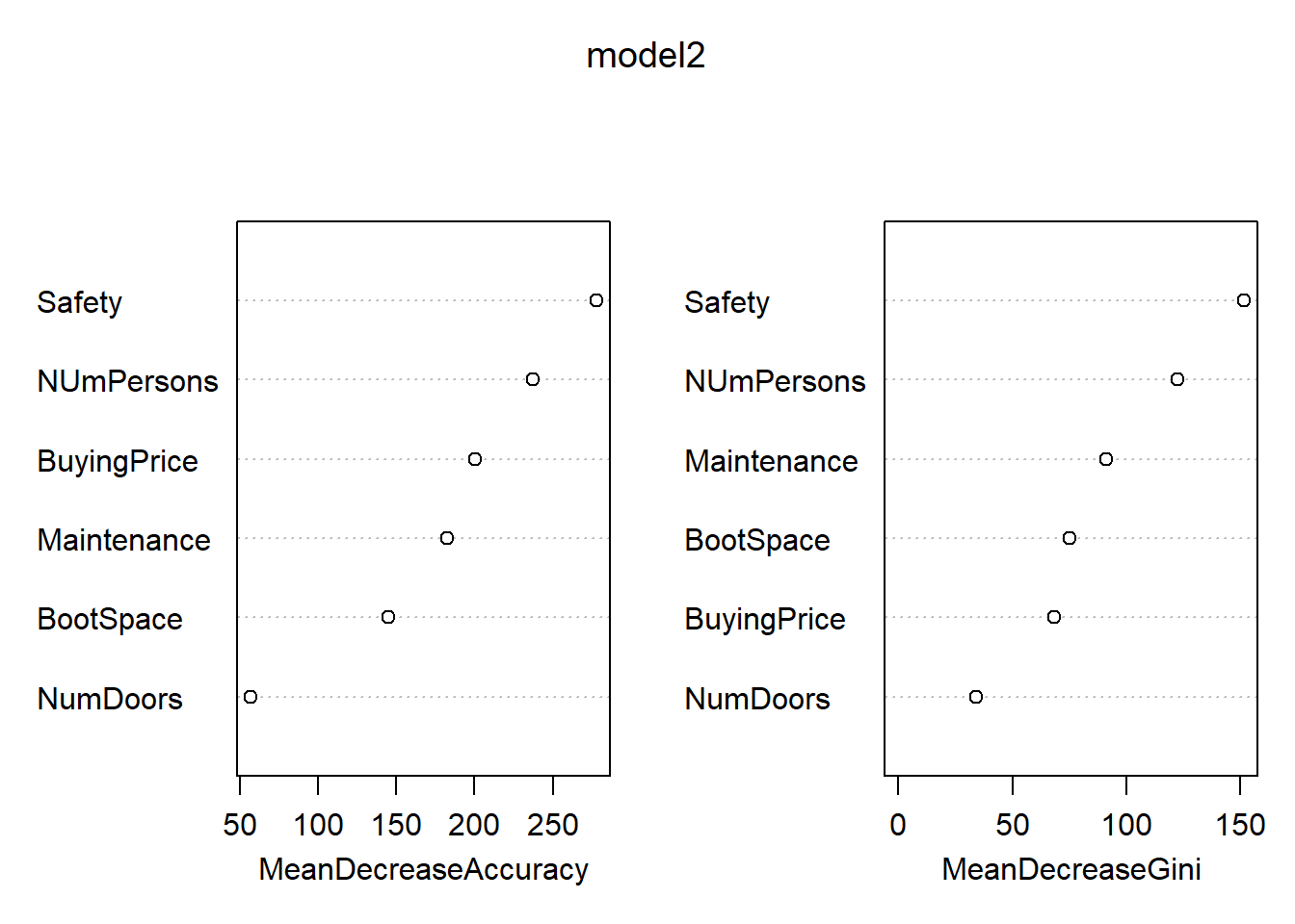
# Using For loop to identify the right mtry for model
a=c()
i=5
for (i in 3:8) {
  model3 <- randomForest(Condition ~ ., data = TrainSet, ntree = 500, mtry = i, importance = TRUE)
  predValid <- predict(model3, ValidSet, type = "class")
  a[i-2] = mean(predValid == ValidSet$Condition)
}
## Warning in randomForest.default(m, y, ...): invalid mtry: reset to within valid
## range

## Warning in randomForest.default(m, y, ...): invalid mtry: reset to within valid
## range

a
## [1] 0.9730250 0.9788054 0.9749518 0.9826590 0.9826590 0.9807322

plot(3:8,a)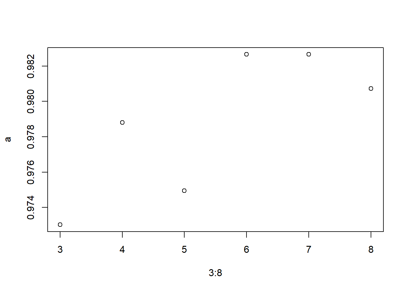
library(rpart)
library(caret)
## Carregando pacotes exigidos: lattice
## Carregando pacotes exigidos: ggplot2
##
## Attaching package: 'ggplot2'
## The following object is masked from 'package:randomForest':
##
##     margin
library(e1071)

# We will compare model 1 of Random Forest with Decision Tree model

model_dt = train(Condition ~ ., data = TrainSet, method = "rpart")
model_dt_1 = predict(model_dt, data = TrainSet)
table(model_dt_1, TrainSet$Condition)
##
## model_dt_1 acc good unacc vgood
##      acc   202   38    75    47
##      good    0    0     0     0
##      unacc  58    8   781     0
##      vgood   0    0     0     0

mean(model_dt_1 == TrainSet$Condition)
## [1] 0.8130687
# Running on Validation Set
model_dt_vs = predict(model_dt, newdata = ValidSet)
table(model_dt_vs, ValidSet$Condition)
##
## model_dt_vs acc good unacc vgood
## acc 101 22 41 18
## good 0 0 0 0
## unacc 23 1 313 0
## vgood 0 0 0 0
mean(model_dt_vs == ValidSet$Condition)
## [1] 0.7976879