1.1 - Recognizing a road sign with kNN

After several trips with a human behind the wheel, it is time for the self-driving car to attempt the test course alone.

As it begins to drive away, its camera captures the following image:

Figure 1: A caption

Can you apply a kNN classifier to help the car recognize this sign?

The dataset signs must be loaded in your workspace along with the dataframe next_sign, which holds the observation you want to classify.

library(class)
## Warning: package 'class' was built under R version 3.6.3

signs <- read.csv(file = "/data_fintech_solutions/knn_traffic_signs.csv", header = TRUE, sep = ",")

dim(signs)
## [1] 206  51

names(signs)
##  [1] "id"        "sample"    "sign_type" "r1"        "g1"        "b1"       
##  [7] "r2"        "g2"        "b2"        "r3"        "g3"        "b3"       
## [13] "r4"        "g4"        "b4"        "r5"        "g5"        "b5"       
## [19] "r6"        "g6"        "b6"        "r7"        "g7"        "b7"       
## [25] "r8"        "g8"        "b8"        "r9"        "g9"        "b9"       
## [31] "r10"       "g10"       "b10"       "r11"       "g11"       "b11"      
## [37] "r12"       "g12"       "b12"       "r13"       "g13"       "b13"      
## [43] "r14"       "g14"       "b14"       "r15"       "g15"       "b15"      
## [49] "r16"       "g16"       "b16"

# get the number of observations
n_obs <- nrow(signs)

# Shuffle row indices: permuted_rows
permuted_rows <- sample(n_obs)

# Randomly order data: signs_shuffled
signs_shuffled <- signs[permuted_rows, ]

# Identify row to split on: split
split <- round(n_obs * 0.7)

# Create train
train <- signs_shuffled[1:split, 3:51]

# Create test
test <- signs_shuffled[(split + 1):n_obs, 3:51]

# Create a vector of labels
sign_types <- signs_shuffled$sign_type[1:split]

next_sign <- signs_shuffled[206, 3:51]

# Classify the next sign observed
signs_pred <- knn(train = train[-1], test = test[-1], cl = sign_types)

You have just trained your first nearest neighbor classifier!

1.2 - Thinking like kNN

With your help, the test car successfully identified the sign and stopped safely at the intersection.

How did the knn() function correctly classify the stop sign?

It was happened because the sign was in some way similar to another stop sign. In fact, kNN learning anytyhing! It simply looks for the most similar example.

1.3 - Exploring the traffic sign dataset

To better understand how the knn() function was able to classify the stop sign, it may help to examine the training dataset it used.

Each previously observed street sign was divided into a 4x4 grid, and the red, green, and blue level for each of the 16 center pixels is recorded as illustrated here.

Figure 2: A caption

The result is a dataset that records the sign_type as well as 16 x 3 = 48 color properties of each sign.

# Examine the structure of the signs dataset
str(signs)
## 'data.frame':    206 obs. of  51 variables:
##  $ id       : int  1 2 3 4 5 6 7 8 9 10 ...
##  $ sample   : Factor w/ 3 levels "example","test",..: 3 3 3 3 3 3 3 2 3 3 ...
##  $ sign_type: Factor w/ 3 levels "pedestrian","speed",..: 1 1 1 1 1 1 1 1 1 1 ...
##  $ r1       : int  155 142 57 22 169 75 136 118 149 13 ...
##  $ g1       : int  228 217 54 35 179 67 149 105 225 34 ...
##  $ b1       : int  251 242 50 41 170 60 157 69 241 28 ...
##  $ r2       : int  135 166 187 171 231 131 200 244 34 5 ...
##  $ g2       : int  188 204 201 178 254 89 203 245 45 21 ...
##  $ b2       : int  101 44 68 26 27 53 107 67 1 11 ...
##  $ r3       : int  156 142 51 19 97 214 150 132 155 123 ...
##  $ g3       : int  227 217 51 27 107 144 167 123 226 154 ...
##  $ b3       : int  245 242 45 29 99 75 134 12 238 140 ...
##  $ r4       : int  145 147 59 19 123 156 171 138 147 21 ...
##  $ g4       : int  211 219 62 27 147 169 218 123 222 46 ...
##  $ b4       : int  228 242 65 29 152 190 252 85 242 41 ...
##  $ r5       : int  166 164 156 42 221 67 171 254 170 36 ...
##  $ g5       : int  233 228 171 37 236 50 158 254 191 60 ...
##  $ b5       : int  245 229 50 3 117 36 108 92 113 26 ...
##  $ r6       : int  212 84 254 217 205 37 157 241 26 75 ...
##  $ g6       : int  254 116 255 228 225 36 186 240 37 108 ...
##  $ b6       : int  52 17 36 19 80 42 11 108 12 44 ...
##  $ r7       : int  212 217 211 221 235 44 26 254 34 13 ...
##  $ g7       : int  254 254 226 235 254 42 35 254 45 27 ...
##  $ b7       : int  11 26 70 20 60 44 10 99 19 25 ...
##  $ r8       : int  188 155 78 181 90 192 180 108 221 133 ...
##  $ g8       : int  229 203 73 183 110 131 211 106 249 163 ...
##  $ b8       : int  117 128 64 73 9 73 236 27 184 126 ...
##  $ r9       : int  170 213 220 237 216 123 129 135 226 83 ...
##  $ g9       : int  216 253 234 234 236 74 109 123 246 125 ...
##  $ b9       : int  120 51 59 44 66 22 73 40 59 19 ...
##  $ r10      : int  211 217 254 251 229 36 161 254 30 13 ...
##  $ g10      : int  254 255 255 254 255 34 190 254 40 27 ...
##  $ b10      : int  3 21 51 2 12 37 10 115 34 25 ...
##  $ r11      : int  212 217 253 235 235 44 161 254 34 9 ...
##  $ g11      : int  254 255 255 243 254 42 190 254 44 23 ...
##  $ b11      : int  19 21 44 12 60 44 6 99 35 18 ...
##  $ r12      : int  172 158 66 19 163 197 187 138 241 85 ...
##  $ g12      : int  235 225 68 27 168 114 215 123 255 128 ...
##  $ b12      : int  244 237 68 29 152 21 236 85 54 21 ...
##  $ r13      : int  172 164 69 20 124 171 141 118 205 83 ...
##  $ g13      : int  235 227 65 29 117 102 142 105 229 125 ...
##  $ b13      : int  244 237 59 34 91 26 140 75 46 19 ...
##  $ r14      : int  172 182 76 64 188 197 189 131 226 85 ...
##  $ g14      : int  228 228 84 61 205 114 171 124 246 128 ...
##  $ b14      : int  235 143 22 4 78 21 140 5 59 21 ...
##  $ r15      : int  177 171 82 211 125 123 214 106 235 85 ...
##  $ g15      : int  235 228 93 222 147 74 221 94 252 128 ...
##  $ b15      : int  244 196 17 78 20 22 201 53 67 21 ...
##  $ r16      : int  22 164 58 19 160 180 188 101 237 83 ...
##  $ g16      : int  52 227 60 27 183 107 211 91 254 125 ...
##  $ b16      : int  53 237 60 29 187 26 227 59 53 19 ...

# Count the number of signs of each type
table(signs$sign_type)
## 
## pedestrian      speed       stop 
##         65         70         71

# Check r10's average red level by sign type
aggregate(r10 ~ sign_type, data = signs, mean)
##    sign_type       r10
## 1 pedestrian 108.78462
## 2      speed  83.08571
## 3       stop 142.50704

As you might have expected, stop signs tend to have a higher average red value. This is how kNN identifies similar signs.

1.4 - Classifying a collection of road signs

Now that the autonomous vehicle has successfully stopped on its own, your team feels confident allowing the car to continue the test course.

The test course includes 59 additional road signs divided into three types:

Figure 3: A caption

Figure 4: A caption

Figure 5: A caption

At the conclusion of the trial, you are asked to measure the car’s overall performance at recognizing these signs.

So is the dataframe test_signs, which holds a set of observations you’ll test your model on.

# Create a confusion matrix of the predicted versus actual values
signs_actual <- test$sign_type
table(signs_actual, signs_pred)
##             signs_pred
## signs_actual pedestrian speed stop
##   pedestrian         18     2    0
##   speed               0    21    1
##   stop                0     0   20

# Compute the accuracy
mean(signs_actual == signs_pred)
## [1] 0.9516129

That self-driving car is really coming along! The confusion matrix lets you look for patterns in the classifier’s

1.5 - Understanding the impact of ‘k’

There is a complex relationship between k and classification accuracy. Bigger is not always better.

Which of these is a valid reason for keeping k as small as possible (but no smaller)?

A smaller k may utilize more subtle patterns.

1.6 - Testing other ‘k’ values

By default, the knn() function in the class package uses only the single nearest neighbor.

Setting a k parameter allows the algorithm to consider additional nearby neighbors. This enlarges the collection of neighbors which will vote on the predicted class.

Compare k values of 1, 7, and 15 to examine the impact on traffic sign classification accuracy.

The class package is already loaded in your workspace along with the datasets signs, signs_test, and sign_types. The object signs_actual holds the true values of the signs.

# Compute the accuracy of the baseline model (default k = 1)
k_1 <- knn(train = train[-1], test = test[-1], cl = sign_types)
mean(signs_actual == k_1)
## [1] 0.9516129

# Modify the above to set k = 7
k_7 <- knn(train = train[-1], test = test[-1], cl = sign_types, k = 7)
mean(signs_actual == k_7)
## [1] 0.9354839

# Set k = 15 and compare to the above
k_15 <- knn(train = train[-1], test = test[-1], cl = sign_types, k = 15)
mean(signs_actual == k_15)
## [1] 0.8870968

1.7 - Seeing how the neighbors voted

When multiple nearest neighbors hold a vote, it can sometimes be useful to examine whether the voters were unanimous or widely separated.

For example, knowing more about the voters’ confidence in the classification could allow an autonomous vehicle to use caution in the case there is any chance at all that a stop sign is ahead.

In this exercise, you will learn how to obtain the voting results from the knn() function.

# Use the prob parameter to get the proportion of votes for the winning class
sign_pred <- knn(train = train[-1], test = test[-1], cl= sign_types, k = 7, prob = TRUE)

# Get the "prob" attribute from the predicted classes
sign_prob <- attr(sign_pred, "prob")

# Examine the first several predictions
head(sign_pred)
## [1] stop  speed stop  stop  speed stop 
## Levels: pedestrian speed stop

# Examine the proportion of votes for the winning class
head(sign_prob)
## [1] 1.0000000 1.0000000 1.0000000 0.5714286 0.8571429 0.4285714

Wow! Awesome job! Now you can get an idea of how certain your kNN learner is about its classifications.

1.8 - Why normalize data?

Before applying kNN to a classification task, it is common practice to rescale the data using a technique like min-max normalization. What is the purpose of this step?

It is to ensure all data elements may contribute equal shares to distance. Rescaling reduces the influence of extreme values on kNN’s distance function.

2.1 - Understanding dependent events

In the previous exercise, you found that there is a 26% chance Brett is in the office at 9am given that it is a weekday.

The events do not overlap, knowing that one occurred tells you much about the status of the other.

2.2 - A simple Naive Bayes location model

The previous exercises showed that the probability that Brett is at work or at home at 9am is highly dependent on whether it is the weekend or a weekday.

To see this finding in action, use the where9am data frame to build a Naive Bayes model on the same data.

You can then use this model to predict the future: where does the model think that Brett will be at 9am on Thursday and at 9am on Saturday?

thursday9am <- data.frame(weekday = "thursday", stringsAsFactors = FALSE)

saturday9am <- data.frame(weekday = "saturday", stringsAsFactors = FALSE)

# Load the naivebayes package
library(naivebayes)
## Warning: package 'naivebayes' was built under R version 3.6.3
## naivebayes 0.9.7 loaded

# Build the location prediction model
locmodel <- naive_bayes(location ~ weekday, data = where9am, laplace = 1)

# Predict Thursday's 9am location
predict(locmodel, thursday9am)
## [1] home
## Levels: appointment campus home office restaurant store theater

# Predict Saturdays's 9am location
predict(locmodel, saturday9am)
## [1] home
## Levels: appointment campus home office restaurant store theater

Awesome job! Not surprisingly, Brett is most likely at the office at 9am on a Thursday, but at home at the same time on a Saturday!

2.3 - Examining “raw” probabilities

The naivebayes package offers several ways to peek inside a Naive Bayes model.

Typing the name of the model object provides the a priori (overall) and conditional probabilities of each of the model’s predictors. If one were so inclined, you might use these for calculating posterior (predicted) probabilities by hand.

Alternatively, R will compute the posterior probabilities for you if the type = “prob” parameter is supplied to the predict() function.

Using these methods, examine how the model’s predicted 9am location probability varies from day-to-day. The model locmodel that you fit in the previous exercise is in your workspace.

# Examine the location prediction model
print(locmodel)
## 
## ================================== Naive Bayes ================================== 
##  
##  Call: 
## naive_bayes.formula(formula = location ~ weekday, data = where9am, 
##     laplace = 1)
## 
## --------------------------------------------------------------------------------- 
##  
## Laplace smoothing: 1
## 
## --------------------------------------------------------------------------------- 
##  
##  A priori probabilities: 
## 
## appointment      campus        home      office  restaurant       store 
## 0.003663004 0.032967033 0.717948718 0.187728938 0.037087912 0.017857143 
##     theater 
## 0.002747253 
## 
## --------------------------------------------------------------------------------- 
##  
##  Tables: 
## 
## --------------------------------------------------------------------------------- 
##  ::: weekday (Categorical) 
## --------------------------------------------------------------------------------- 
##            
## weekday     appointment      campus        home      office  restaurant
##   friday    0.133333333 0.189873418 0.121269841 0.182254197 0.238636364
##   monday    0.133333333 0.189873418 0.126984127 0.206235012 0.113636364
##   saturday  0.333333333 0.012658228 0.182222222 0.002398082 0.102272727
##   sunday    0.066666667 0.012658228 0.189841270 0.002398082 0.113636364
##   thursday  0.066666667 0.253164557 0.122539683 0.208633094 0.136363636
##   tuesday   0.066666667 0.037974684 0.129523810 0.223021583 0.136363636
##   wednesday 0.200000000 0.303797468 0.127619048 0.175059952 0.159090909
##            
## weekday           store     theater
##   friday    0.282608696 0.076923077
##   monday    0.108695652 0.076923077
##   saturday  0.195652174 0.538461538
##   sunday    0.130434783 0.076923077
##   thursday  0.108695652 0.076923077
##   tuesday   0.108695652 0.076923077
##   wednesday 0.065217391 0.076923077
## 
## ---------------------------------------------------------------------------------

# Obtain the predicted probabilities for Thursday at 9am
predict(locmodel, thursday9am, type = "prob")
##      appointment    campus      home    office restaurant      store
## [1,] 0.001708366 0.0583872 0.6154674 0.2739992 0.03538065 0.01357873
##          theater
## [1,] 0.001478394

# Obtain the predicted probabilities for Saturday at 9am
predict(locmodel, saturday9am, type = "prob")
##      appointment      campus      home      office restaurant      store
## [1,] 0.008617968 0.002945382 0.9233866 0.003177488 0.02677201 0.02465957
##       theater
## [1,] 0.010441

Fantastic! Did you notice the predicted probability of Brett being at the office on a Saturday is almost zero?

2.4 - Understanding independence

Understanding the idea of event independence will become important as you learn more about how “naive” Bayes got its name. Which of the following is true about independent events?

Knowing the outcome of one event does not help predict the other. Yes! One event is independent of another if knowing one doesn’t give you information about how likely the other is. For example, knowing if it’s raining in New York doesn’t help you predict the weather in San Francisco. The weather events in the two cities are independent of each other.

2.5 - Who are you calling naive?

The Naive Bayes algorithm got its name because it makes a “naive” assumption about event independence.

What is the purpose of making this assumption? The joint probability calculations is simpler for independent events. The joint probability of independent events can be computed much more simply by multiplying their individual probabilities

2.6 - A more sophisticated location model

The locations dataset (where9am) records Brett’s location every hour for 13 weeks. Each hour, the tracking information includes the daytype (weekend or weekday) as well as the hourtype (morning, afternoon, evening, or night).

Using this data, build a more sophisticated model to see how Brett’s predicted location not only varies by the day of week but also by the time of day.

You can specify additional independent variables in your formula using the + sign (e.g. y ~ x + b).

weekday_afternoon <- data.frame(daytype = "weekday",
                                hourtype = "afternoon",
                                location = "office", stringsAsFactors = FALSE)

weekday_evening <- data.frame(daytype = "weekday",
                                hourtype = "evening",
                                location = "home", stringsAsFactors = FALSE)

# Build a NB model of location
locmodel <- naive_bayes(location ~ daytype + hourtype, where9am, laplace = 0)
## Warning: naive_bayes(): Feature daytype - zero probabilities are present.
## Consider Laplace smoothing.
## Warning: naive_bayes(): Feature hourtype - zero probabilities are present.
## Consider Laplace smoothing.

# Predict Brett's location on a weekday afternoon
predict(locmodel, weekday_afternoon)
## Warning: predict.naive_bayes(): more features in the newdata are provided as
## there are probability tables in the object. Calculation is performed based on
## features to be found in the tables.
## [1] office
## Levels: appointment campus home office restaurant store theater

# Predict Brett's location on a weekday evening
predict(locmodel, weekday_evening)
## Warning: predict.naive_bayes(): more features in the newdata are provided as
## there are probability tables in the object. Calculation is performed based on
## features to be found in the tables.
## [1] home
## Levels: appointment campus home office restaurant store theater

Your Naive Bayes model forecasts that Brett will be at the office on a weekday afternoon and at home in the evening.

2.7 - Preparing for unforeseen circumstances

While Brett was tracking his location over 13 weeks, he never went into the office during the weekend. Consequently, the joint probability of P(office and weekend) = 0.

Explore how this impacts the predicted probability that Brett may go to work on the weekend in the future. Additionally, you can see how using the Laplace correction will allow a small chance for these types of unforeseen circumstances.

weekend_afternoon <- data.frame(daytype = "weekend",
                                hourtype = "afternoon",
                                location = "home", stringsAsFactors = FALSE)

weekend_evening <- data.frame(daytype = "weekend",
                                hourtype = "evening",
                                location = "home", stringsAsFactors = FALSE)

# Observe the predicted probabilities for a weekend afternoon
predict(locmodel, weekend_afternoon, type = "prob")
## Warning: predict.naive_bayes(): more features in the newdata are provided as
## there are probability tables in the object. Calculation is performed based on
## features to be found in the tables.
##      appointment       campus      home      office restaurant      store
## [1,]  0.02462883 0.0004802622 0.8439145 0.003349521  0.1111338 0.01641922
##          theater
## [1,] 7.38865e-05

# Build a new model using the Laplace correction
locmodel2 <- naive_bayes(location ~ daytype + hourtype, where9am, laplace = 1)

# Observe the new predicted probabilities for a weekend afternoon
predict(locmodel2, weekend_afternoon, type = "prob")
## Warning: predict.naive_bayes(): more features in the newdata are provided as
## there are probability tables in the object. Calculation is performed based on
## features to be found in the tables.
##      appointment      campus      home      office restaurant      store
## [1,]  0.02013872 0.006187715 0.8308154 0.007929249  0.1098743 0.01871085
##          theater
## [1,] 0.006343697

Fantastic work! Adding the Laplace correction allows for the small chance that Brett might go to the office on the weekend in the future.

2.8 - Understanding the Laplace correction

By default, the naive_bayes function in the naivebayes packahe does not use the Laplace correction. What is the risk of leaving this parameter unset?

Some potential outcomes may be predicted to be impossible. The small probability added to every outcome ensures that they are all possible even if never previously observed.

3.1 - Building simple logistic regression models

The donors dataset contains 93,462 examples of people mailed in a fundraising solicitation for paralyzed military veterans. The donated column is 1 if the person made a donation in response to the mailing and 0 otherwise. This binary outcome will be the dependent variable for the logistic regression model.

The remaining columns are features of the prospective donors that may influence their donation behavior. These are the model’s independent variables.

When building a regression model, it is often helpful to form a hypothesis about which independent variables will be predictive of the dependent variable. The bad_address column, which is set to 1 for an invalid mailing address and 0 otherwise, seems like it might reduce the chances of a donation. Similarly, one might suspect that religious interest (interest_religion) and interest in veterans affairs (interest_veterans) would be associated with greater charitable giving.

In this exercise, you will use these three factors to create a simple model of donation behavior. The dataset donors is available in your workspace.

donors <- read.csv(file = "/data_fintech_solutions/donors.csv", header = TRUE, sep = ",")

# Examine the dataset to identify potential independent variables
str(donors)
## 'data.frame':    93462 obs. of  13 variables:
##  $ donated          : int  0 0 0 0 0 0 0 0 0 0 ...
##  $ veteran          : int  0 0 0 0 0 0 0 0 0 0 ...
##  $ bad_address      : int  0 0 0 0 0 0 0 0 0 0 ...
##  $ age              : int  60 46 NA 70 78 NA 38 NA NA 65 ...
##  $ has_children     : int  0 1 0 0 1 0 1 0 0 0 ...
##  $ wealth_rating    : int  0 3 1 2 1 0 2 3 1 0 ...
##  $ interest_veterans: int  0 0 0 0 0 0 0 0 0 0 ...
##  $ interest_religion: int  0 0 0 0 1 0 0 0 0 0 ...
##  $ pet_owner        : int  0 0 0 0 0 0 1 0 0 0 ...
##  $ catalog_shopper  : int  0 0 0 0 1 0 0 0 0 0 ...
##  $ recency          : Factor w/ 2 levels "CURRENT","LAPSED": 1 1 1 1 1 1 1 1 1 1 ...
##  $ frequency        : Factor w/ 2 levels "FREQUENT","INFREQUENT": 1 1 1 1 1 2 2 1 2 2 ...
##  $ money            : Factor w/ 2 levels "HIGH","MEDIUM": 2 1 2 2 2 2 2 2 2 2 ...

# Explore the dependent variable
table(donors$donated)
## 
##     0     1 
## 88751  4711

# Build the donation model
donation_model <- glm(donated ~ bad_address + interest_religion + interest_veterans, 
                      data = donors, family = "binomial")

# Summarize the model results
summary(donation_model)
## 
## Call:
## glm(formula = donated ~ bad_address + interest_religion + interest_veterans, 
##     family = "binomial", data = donors)
## 
## Deviance Residuals: 
##     Min       1Q   Median       3Q      Max  
## -0.3480  -0.3192  -0.3192  -0.3192   2.5678  
## 
## Coefficients:
##                   Estimate Std. Error  z value Pr(>|z|)    
## (Intercept)       -2.95139    0.01652 -178.664   <2e-16 ***
## bad_address       -0.30780    0.14348   -2.145   0.0319 *  
## interest_religion  0.06724    0.05069    1.327   0.1847    
## interest_veterans  0.11009    0.04676    2.354   0.0186 *  
## ---
## Signif. codes:  0 '***' 0.001 '**' 0.01 '*' 0.05 '.' 0.1 ' ' 1
## 
## (Dispersion parameter for binomial family taken to be 1)
## 
##     Null deviance: 37330  on 93461  degrees of freedom
## Residual deviance: 37316  on 93458  degrees of freedom
## AIC: 37324
## 
## Number of Fisher Scoring iterations: 5

Great work! With the model built, you can now use it to make predictions!

3.2 - Making a binary prediction

In the previous exercise, you used the glm() function to build a logistic regression model of donor behavior. As with many of R’s machine learning methods, you can apply the predict() function to the model object to forecast future behavior. By default, predict() outputs predictions in terms of log odds unless type = “response” is specified. This converts the log odds to probabilities.

Because a logistic regression model estimates the probability of the outcome, it is up to you to determine the threshold at which the probability implies action. One must balance the extremes of being too cautious versus being too aggressive. For example, if you were to solicit only the people with a 99% or greater donation probability, you may miss out on many people with lower estimated probabilities that still choose to donate. This balance is particularly important to consider for severely imbalanced outcomes, such as in this dataset where donations are relatively rare.

# Estimate the donation probability
donors$donation_prob <- predict(donation_model, type = "response")

# Find the donation probability of the average prospect
mean(donors$donated)
## [1] 0.05040551

# Predict a donation if probability of donation is greater than average (0.0504)
donors$donation_pred <- ifelse(donors$donation_prob > 0.0504, 1, 0)

# Calculate the model's accuracy
mean(donors$donation_pred == donors$donated)
## [1] 0.794815

Nice work! With an accuracy of nearly 80%, the model seems to be doing its job. But is it too good to be true?

3.3 - The limitations of accuracy

In the previous exercise, you found that the logistic regression model made a correct prediction nearly 80% of the time. Despite this relatively high accuracy, the result is misleading due to the rarity of outcome being predicted.

What would the accuracy have been if a model had simply predicted “no donation” for each person?

library(dplyr)
## Warning: package 'dplyr' was built under R version 3.6.3
## 
## Attaching package: 'dplyr'
## The following objects are masked from 'package:stats':
## 
##     filter, lag
## The following objects are masked from 'package:base':
## 
##     intersect, setdiff, setequal, union
prop <- table(donors$donated)
round(prop.table(prop) * 100, 3)
## 
##      0      1 
## 94.959  5.041

With an accuracy of only 80%, the model is actually performing WORSE than if it were to predict non-donor for every record.

3.4 - Calculating ROC Curves and AUC

One good way to assess classifiers in binaries problems is analysing and implementing ROC Curves (Receiving Operating Characteristics).

The previous exercises have demonstrated that accuracy is a very misleading measure of model performance on imbalanced datasets. Graphing the model’s performance better illustrates the tradeoff between a model that is overly agressive and one that is overly passive.

In this exercise you will create a ROC curve and compute the area under the curve (AUC) to evaluate the logistic regression model of donations you built earlier.

The dataset donors with the column of predicted probabilities, donation_prob.

# Load the pROC package
library(pROC)
## Warning: package 'pROC' was built under R version 3.6.3
## Type 'citation("pROC")' for a citation.
## 
## Attaching package: 'pROC'
## The following objects are masked from 'package:stats':
## 
##     cov, smooth, var

# Create a ROC curve
ROC <- roc(donors$donated, donors$donation_prob)
## Setting levels: control = 0, case = 1
## Setting direction: controls < cases

# Plot the ROC curve
plot(ROC, col = "blue")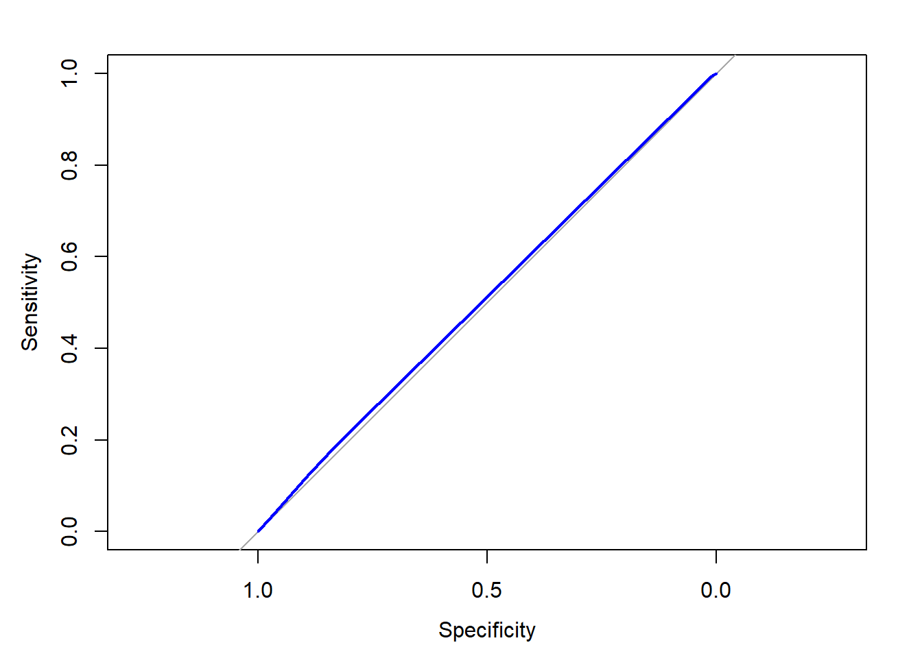

# Calculate the area under the curve (AUC)
auc(ROC)
## Area under the curve: 0.5102

Awesome job! Based on this visualization, the model isn’t doing much better than baseline— a model doing nothing but making predictions at random.

3.5 - Comparing ROC (Receiving Operating Characteristics) curves

Which of the following ROC curves illustrates the best model?

Figure 6: A caption

When AUC (Area under the Curve) values are very close, it’s important to know more about how the model will be used.

3.6 - Coding categorical features

Sometimes a dataset contains numeric values that represent a categorical feature.

In the donors dataset, wealth_rating uses numbers to indicate the donor’s wealth level:

0 = Unknown 1 = Low 2 = Medium 3 = High This exercise illustrates how to prepare this type of categorical feature and examines its impact on a logistic regression model.

# Convert the wealth rating to a factor
donors$wealth_levels <- factor(donors$wealth_rating, levels = c(0, 1, 2, 3), labels = c("Unknown", "Low", "Medium", "High"))

# Use relevel() to change reference category
donors$wealth_levels <- relevel(donors$wealth_levels, ref = "Medium")

# See how our factor coding impacts the model
summary(glm(donated ~ wealth_levels, donors, family = "binomial"))
## 
## Call:
## glm(formula = donated ~ wealth_levels, family = "binomial", data = donors)
## 
## Deviance Residuals: 
##     Min       1Q   Median       3Q      Max  
## -0.3320  -0.3243  -0.3175  -0.3175   2.4582  
## 
## Coefficients:
##                      Estimate Std. Error z value Pr(>|z|)    
## (Intercept)          -2.91894    0.03614 -80.772   <2e-16 ***
## wealth_levelsUnknown -0.04373    0.04243  -1.031    0.303    
## wealth_levelsLow     -0.05245    0.05332  -0.984    0.325    
## wealth_levelsHigh     0.04804    0.04768   1.008    0.314    
## ---
## Signif. codes:  0 '***' 0.001 '**' 0.01 '*' 0.05 '.' 0.1 ' ' 1
## 
## (Dispersion parameter for binomial family taken to be 1)
## 
##     Null deviance: 37330  on 93461  degrees of freedom
## Residual deviance: 37323  on 93458  degrees of freedom
## AIC: 37331
## 
## Number of Fisher Scoring iterations: 5

Great job! What would the model output have looked like if this variable had been left as a numeric column?

3.7 - Handling missing data

Some of the prospective donors have missing age data. Unfortunately, R will exclude any cases with NA values when building a regression model.

One workaround is to replace, or impute, the missing values with an estimated value. After doing so, you may also create a missing data indicator to model the possibility that cases with missing data are different in some way from those without.

summary(donors$age)
##    Min. 1st Qu.  Median    Mean 3rd Qu.    Max.    NA's 
##    1.00   48.00   62.00   61.65   75.00   98.00   22546

# Find the average age among non-missing values
summary(donors$age)
##    Min. 1st Qu.  Median    Mean 3rd Qu.    Max.    NA's 
##    1.00   48.00   62.00   61.65   75.00   98.00   22546

# Impute missing age values with the mean age
donors$imputed_age <- ifelse(is.na(donors$age), round(mean(donors$age, na.rm = TRUE), 2), donors$age)

# Create missing value indicator for age
donors$missing_age <- ifelse(is.na(donors$age), 1, 0)

Super! This is one way to handle missing data, but be careful! Sometimes missing data has to be dealt with using more complicated methods.

3.8 - Understanding missing value indicators

A missing value indicator provides a reminder that, before imputation, there was a missing value present on the record.

Why is it often useful to include this indicator as a predictor in the model? It is useful for these reasons:

• A missing value may represent a unique category by itself
• There may be an important difference between records with and without missing data
• Whatever caused the missing value may also be related to the outcome

Sometimes a missing value says a great deal about the record it appeared on!

3.9 - Building a more sophisticated model

One of the best predictors of future giving is a history of recent, frequent, and large gifts. In marketing terms, this is known as R/F/M:

• Recency
• Frequency
• Money

Donors that haven’t given both recently and frequently may be especially likely to give again; in other words, the combined impact of recency and frequency may be greater than the sum of the separate effects.

Because these predictors together have a greater impact on the dependent variable, their joint effect must be modeled as an interaction.

# Build a recency, frequency, and money (RFM) model
rfm_model <- glm(donated ~ money + recency * frequency, family = "binomial", donors)

# Summarize the RFM model to see how the parameters were coded
summary(rfm_model)
## 
## Call:
## glm(formula = donated ~ money + recency * frequency, family = "binomial", 
##     data = donors)
## 
## Deviance Residuals: 
##     Min       1Q   Median       3Q      Max  
## -0.3696  -0.3696  -0.2895  -0.2895   2.7924  
## 
## Coefficients:
##                                   Estimate Std. Error z value Pr(>|z|)    
## (Intercept)                       -3.01142    0.04279 -70.375   <2e-16 ***
## moneyMEDIUM                        0.36186    0.04300   8.415   <2e-16 ***
## recencyLAPSED                     -0.86677    0.41434  -2.092   0.0364 *  
## frequencyINFREQUENT               -0.50148    0.03107 -16.143   <2e-16 ***
## recencyLAPSED:frequencyINFREQUENT  1.01787    0.51713   1.968   0.0490 *  
## ---
## Signif. codes:  0 '***' 0.001 '**' 0.01 '*' 0.05 '.' 0.1 ' ' 1
## 
## (Dispersion parameter for binomial family taken to be 1)
## 
##     Null deviance: 37330  on 93461  degrees of freedom
## Residual deviance: 36938  on 93457  degrees of freedom
## AIC: 36948
## 
## Number of Fisher Scoring iterations: 6

# Compute predicted probabilities for the RFM model
rfm_prob <- predict(rfm_model, type = "response")

# Plot the ROC curve and find AUC for the new model
library(pROC)
ROC <- roc(donors$donated, rfm_prob)
## Setting levels: control = 0, case = 1
## Setting direction: controls < cases
plot(ROC, col = "red")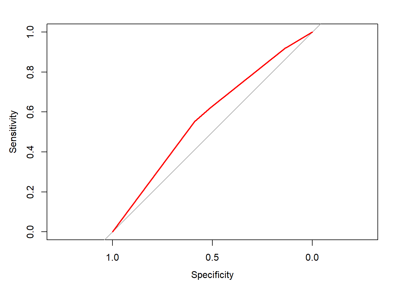

auc(ROC)
## Area under the curve: 0.5785

Great work! Based on the ROC curve, you’ve confirmed that past giving patterns are certainly predictive of future giving.

3.10 - The dangers of stepwise regression

In spite of its utility for feature selection, stepwise regression is not frequently used in disciplines outside of machine learning due to some important caveats. Though stepwise regression is frowned upon, it may still be useful for building predictive models in the absence of another starting place.

3.11 - Building a stepwise regression model

In the absence of subject-matter expertise, stepwise regression can assist with the search for the most important predictors of the outcome of interest.

In this exercise, you will use a forward stepwise approach to add predictors to the model one-by-one until no additional benefit is seen.

# Specify a null model with no predictors
null_model <- glm(donated ~ 1, data = donors, family = "binomial")

# Specify the full model using all of the potential predictors
full_model <- glm(donated ~ ., donors, family= "binomial")

# Use a forward stepwise algorithm to build a parsimonious model
step_model <- step(null_model, scope = list(lower = null_model, upper = full_model), direction = "forward")
## Start:  AIC=37332.13
## donated ~ 1
## Warning in add1.glm(fit, scope$add, scale = scale, trace = trace, k = k, : using
## the 70916/93462 rows from a combined fit
##                     Df Deviance   AIC
## + frequency          1    28502 37122
## + money              1    28621 37241
## + wealth_rating      1    28705 37326
## + has_children       1    28705 37326
## + age                1    28707 37328
## + imputed_age        1    28707 37328
## + wealth_levels      3    28704 37328
## + interest_veterans  1    28709 37330
## + donation_prob      1    28710 37330
## + donation_pred      1    28710 37330
## + catalog_shopper    1    28710 37330
## + pet_owner          1    28711 37331
## <none>                    28714 37332
## + interest_religion  1    28712 37333
## + recency            1    28713 37333
## + bad_address        1    28714 37334
## + veteran            1    28714 37334
## 
## Step:  AIC=37024.77
## donated ~ frequency
## Warning in add1.glm(fit, scope$add, scale = scale, trace = trace, k = k, : using
## the 70916/93462 rows from a combined fit
##                     Df Deviance   AIC
## + money              1    28441 36966
## + wealth_rating      1    28493 37018
## + wealth_levels      3    28490 37019
## + has_children       1    28494 37019
## + donation_prob      1    28498 37023
## + interest_veterans  1    28498 37023
## + catalog_shopper    1    28499 37024
## + donation_pred      1    28499 37024
## + age                1    28499 37024
## + imputed_age        1    28499 37024
## + pet_owner          1    28499 37024
## <none>                    28502 37025
## + interest_religion  1    28501 37026
## + recency            1    28501 37026
## + bad_address        1    28502 37026
## + veteran            1    28502 37027
## 
## Step:  AIC=36949.71
## donated ~ frequency + money
## Warning in add1.glm(fit, scope$add, scale = scale, trace = trace, k = k, : using
## the 70916/93462 rows from a combined fit
##                     Df Deviance   AIC
## + wealth_levels      3    28427 36942
## + wealth_rating      1    28431 36942
## + has_children       1    28432 36943
## + interest_veterans  1    28438 36948
## + donation_prob      1    28438 36949
## + catalog_shopper    1    28438 36949
## + donation_pred      1    28439 36949
## + age                1    28439 36949
## + imputed_age        1    28439 36949
## + pet_owner          1    28439 36949
## <none>                    28441 36950
## + interest_religion  1    28440 36951
## + recency            1    28441 36951
## + bad_address        1    28441 36951
## + veteran            1    28441 36952
## 
## Step:  AIC=36945.48
## donated ~ frequency + money + wealth_levels
## Warning in add1.glm(fit, scope$add, scale = scale, trace = trace, k = k, : using
## the 70916/93462 rows from a combined fit
##                     Df Deviance   AIC
## + has_children       1    28416 36937
## + age                1    28424 36944
## + imputed_age        1    28424 36944
## + interest_veterans  1    28424 36945
## + donation_prob      1    28424 36945
## + catalog_shopper    1    28425 36945
## + donation_pred      1    28425 36945
## <none>                    28427 36945
## + pet_owner          1    28425 36946
## + interest_religion  1    28426 36947
## + recency            1    28427 36947
## + bad_address        1    28427 36947
## + veteran            1    28427 36947
## 
## Step:  AIC=36938.4
## donated ~ frequency + money + wealth_levels + has_children
## Warning in add1.glm(fit, scope$add, scale = scale, trace = trace, k = k, : using
## the 70916/93462 rows from a combined fit
##                     Df Deviance   AIC
## + pet_owner          1    28413 36937
## + donation_prob      1    28413 36937
## + catalog_shopper    1    28413 36937
## + interest_veterans  1    28413 36937
## + donation_pred      1    28414 36938
## <none>                    28416 36938
## + interest_religion  1    28415 36939
## + age                1    28416 36940
## + imputed_age        1    28416 36940
## + recency            1    28416 36940
## + bad_address        1    28416 36940
## + veteran            1    28416 36940
## 
## Step:  AIC=36932.25
## donated ~ frequency + money + wealth_levels + has_children + 
##     pet_owner
## Warning in add1.glm(fit, scope$add, scale = scale, trace = trace, k = k, : using
## the 70916/93462 rows from a combined fit
##                     Df Deviance   AIC
## <none>                    28413 36932
## + donation_prob      1    28411 36932
## + interest_veterans  1    28411 36932
## + catalog_shopper    1    28412 36933
## + donation_pred      1    28412 36933
## + age                1    28412 36933
## + imputed_age        1    28412 36933
## + recency            1    28413 36934
## + interest_religion  1    28413 36934
## + bad_address        1    28413 36934
## + veteran            1    28413 36934

# Estimate the stepwise donation probability
step_prob <- predict(step_model, type = "response")

# Plot the ROC of the stepwise model
library(pROC)
ROC <- roc(donors$donated, step_prob)
## Setting levels: control = 0, case = 1
## Setting direction: controls < cases
plot(ROC, col = "red")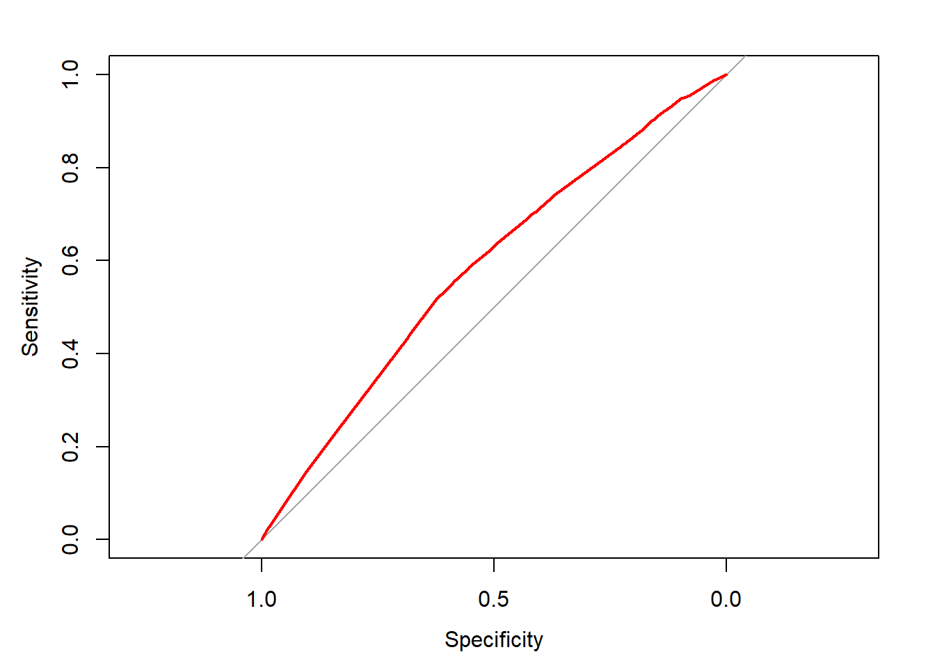

auc(ROC)
## Area under the curve: 0.5849

Fantastic work! Despite the caveats of stepwise regression, it seems to have resulted in a relatively strong model!

Obs.: I strongly recommend that you enrol in one of the DataCamp courses. This content was published in this way as a form to organized my studies in try to do my best in terms of knowledge and discover new trends, ideas or analysis in terms of credit modeling.