By Salerno | May 10, 2022
1) Introduction
It is so straightforward working with the IDE RStudio (in my opinion, one of the most relevant and easy to use) and a connection with a DataBase (in this case we are using PostgreSQL).
Check it out in the lines below one way (of course there are other options) to connect.
Enjoy it!
2) Packages we are using
DBIdplyrodbc
# 2) Important packages ----
library(DBI)
library(dplyr)
library(odbc)
3) Checking out the data sources available
This is one important step that you have to check if the driver that you want was installed in your machine.
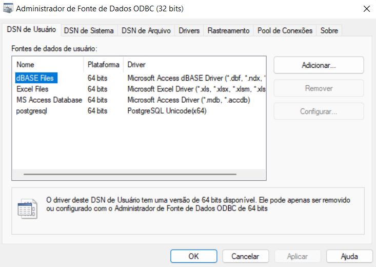
# 3) All data sources ----
data.frame(odbcListDataSources()[[2]][[4]])
##   odbcListDataSources....2....4..
## 1         PostgreSQL Unicode(x64)
4) Selecting a PostgreSQL data source
# 4) Defining a PostgreSQL DS ----
ds_postgresql <- odbcListDataSources()[[1]][4]
5) Listing all drives available
# 5) Checking all drivers ----
drv_all <- sort(unique(odbcListDrivers()[[1]]))
6) Selecting a PostgreSQL driver
# 6) Defining a PostgreSQL drive ----
drv_postgresql <- drv_all[9]
7) Creating a connection with a database
# 7) Connection ----
con <- dbConnect(odbc::odbc(),
                 dsn = ds_postgresql,
                 server = "localhost",
                 uid = "postgres",
                 database= "rstudio_test")
8) Listing objects connected
# 8) Listing Connected Objects ----
odbcListObjects(con)
##           name    type
## 1 rstudio_test catalog
9) Creating a dataframe for test
# 9) An example data frame to play with ----
iris <- as.data.frame(iris)
summary(iris)
##   Sepal.Length    Sepal.Width     Petal.Length    Petal.Width
##  Min.   :4.300   Min.   :2.000   Min.   :1.000   Min.   :0.100
##  1st Qu.:5.100   1st Qu.:2.800   1st Qu.:1.600   1st Qu.:0.300
##  Median :5.800   Median :3.000   Median :4.350   Median :1.300
##  Mean   :5.843   Mean   :3.057   Mean   :3.758   Mean   :1.199
##  3rd Qu.:6.400   3rd Qu.:3.300   3rd Qu.:5.100   3rd Qu.:1.800
##  Max.   :7.900   Max.   :4.400   Max.   :6.900   Max.   :2.500
##        Species
##  setosa    :50
##  versicolor:50
##  virginica :50
##
##
##
10) Adjusting atributes names and writing data in the database
# 10) make names db safe: no '.' or other illegal characters, all lower case and unique ----
dbSafeNames = function(names) {
  names = gsub('[^a-z0-9]+', '_', tolower(names))
  names = make.names(names, unique = TRUE, allow_ = TRUE)
  names = gsub('.', '_', names, fixed = TRUE)
  names
}

colnames(iris) = dbSafeNames(colnames(iris))
summary(iris)
##   sepal_length    sepal_width     petal_length    petal_width
##  Min.   :4.300   Min.   :2.000   Min.   :1.000   Min.   :0.100
##  1st Qu.:5.100   1st Qu.:2.800   1st Qu.:1.600   1st Qu.:0.300
##  Median :5.800   Median :3.000   Median :4.350   Median :1.300
##  Mean   :5.843   Mean   :3.057   Mean   :3.758   Mean   :1.199
##  3rd Qu.:6.400   3rd Qu.:3.300   3rd Qu.:5.100   3rd Qu.:1.800
##  Max.   :7.900   Max.   :4.400   Max.   :6.900   Max.   :2.500
##        species
##  setosa    :50
##  versicolor:50
##  virginica :50
##
##
##

dbWriteTable(con, 'iris', iris, row.names=FALSE)
11) Fetching data from database
11.1) Method 1
# 11.1) Read back the full table: method 1 ----
dtab = dbGetQuery(con, 'select * from iris')
summary(dtab)
##   sepal_length    sepal_width     petal_length    petal_width
##  Min.   :4.300   Min.   :2.000   Min.   :1.000   Min.   :0.100
##  1st Qu.:5.100   1st Qu.:2.800   1st Qu.:1.600   1st Qu.:0.300
##  Median :5.800   Median :3.000   Median :4.350   Median :1.300
##  Mean   :5.843   Mean   :3.057   Mean   :3.758   Mean   :1.199
##  3rd Qu.:6.400   3rd Qu.:3.300   3rd Qu.:5.100   3rd Qu.:1.800
##  Max.   :7.900   Max.   :4.400   Max.   :6.900   Max.   :2.500
##    species
##  Length:150
##  Class :character
##  Mode  :character
##
##
##
11.2) Method 2
# 11.2) Read back the full table: method 2 ----
rm(dtab)
dtab = dbReadTable(con, 'iris')
summary(dtab)
##   sepal_length    sepal_width     petal_length    petal_width
##  Min.   :4.300   Min.   :2.000   Min.   :1.000   Min.   :0.100
##  1st Qu.:5.100   1st Qu.:2.800   1st Qu.:1.600   1st Qu.:0.300
##  Median :5.800   Median :3.000   Median :4.350   Median :1.300
##  Mean   :5.843   Mean   :3.057   Mean   :3.758   Mean   :1.199
##  3rd Qu.:6.400   3rd Qu.:3.300   3rd Qu.:5.100   3rd Qu.:1.800
##  Max.   :7.900   Max.   :4.400   Max.   :6.900   Max.   :2.500
##    species
##  Length:150
##  Class :character
##  Mode  :character
##
##
##
12) Selecting partial data
# 12) Get part of the table ----
rm(dtab)
dtab = dbGetQuery(con, 'select sepal_length, species from iris')
summary(dtab)
##   sepal_length     species
##  Min.   :4.300   Length:150
##  1st Qu.:5.100   Class :character
##  Median :5.800   Mode  :character
##  Mean   :5.843
##  3rd Qu.:6.400
##  Max.   :7.900
13) Using a dplyr for connecting
# 13) Using dplyr package ----
iris <- con %>%
  tbl('iris')

iris <- as.data.frame(iris)

str(iris)
## 'data.frame':	150 obs. of  5 variables:
##  $ sepal_length: num  5.1 4.9 4.7 4.6 5 5.4 4.6 5 4.4 4.9 ...
##  $ sepal_width : num  3.5 3 3.2 3.1 3.6 3.9 3.4 3.4 2.9 3.1 ...
##  $ petal_length: num  1.4 1.4 1.3 1.5 1.4 1.7 1.4 1.5 1.4 1.5 ...
##  $ petal_width : num  0.2 0.2 0.2 0.2 0.2 0.4 0.3 0.2 0.2 0.1 ...
##  $ species     : chr  "setosa" "setosa" "setosa" "setosa" ...
14) Creating a query
# 14) Send a query through dplyr ----
query = "select avg(sepal_length) avg_sepal_length,
                species
         from iris
         group by species"
dsub = tbl(con, sql(query))
dsub
## # Source:   SQL [3 x 2]
## # Database: postgres  [postgres@localhost:/rstudio_test]
##   avg_sepal_length species
##              <dbl> <chr>
## 1             6.59 virginica
## 2             5.94 versicolor
## 3             5.01 setosa
15) Making data avaliable in your local machine
# 15) Make it local ----
dsub = as.data.frame(dsub)
summary(dsub)
##  avg_sepal_length   species
##  Min.   :5.006    Length:3
##  1st Qu.:5.471    Class :character
##  Median :5.936    Mode  :character
##  Mean   :5.843
##  3rd Qu.:6.262
##  Max.   :6.588
16) Removing database
# 16) Remove table from database ----
dbSendQuery(con, "drop table iris")
## <OdbcResult>
##   SQL  drop table iris
##   ROWS Fetched: 0 [complete]
##        Changed: 430835857
17) Closing connection databse
# 17) Disconnect from the database ----
dbDisconnect(con)
## Warning in connection_release(conn@ptr): There is a result object still in use.
## The connection will be automatically released when it is closed
comments powered by Disqus