Linear Regression

Data

We are using the MASS library that contains the Boston dataset. These records measure the median house value for 506 neighborhoods around Boston.

library(MASS)
data <- MASS::Boston
fix(Boston)
names(Boston)
##  [1] "crim"    "zn"      "indus"   "chas"    "nox"     "rm"      "age"    
##  [8] "dis"     "rad"     "tax"     "ptratio" "black"   "lstat"   "medv"

A simple Linear Regression

We are using the lm() function to fit a simple linear regression model. The medv is a response variable and lstat the predictor variable.

The basic syntax is lm(y~x, data).

attach(Boston)
lm.fit = lm(medv~lstat)

lm.fit
## 
## Call:
## lm(formula = medv ~ lstat)
## 
## Coefficients:
## (Intercept)        lstat  
##       34.55        -0.95

cor(lstat, medv)
## [1] -0.7376627

Summary Function

This functio give us some insights about the dataset.

summary(Boston)
##       crim                zn             indus            chas        
##  Min.   : 0.00632   Min.   :  0.00   Min.   : 0.46   Min.   :0.00000  
##  1st Qu.: 0.08204   1st Qu.:  0.00   1st Qu.: 5.19   1st Qu.:0.00000  
##  Median : 0.25651   Median :  0.00   Median : 9.69   Median :0.00000  
##  Mean   : 3.61352   Mean   : 11.36   Mean   :11.14   Mean   :0.06917  
##  3rd Qu.: 3.67708   3rd Qu.: 12.50   3rd Qu.:18.10   3rd Qu.:0.00000  
##  Max.   :88.97620   Max.   :100.00   Max.   :27.74   Max.   :1.00000  
##       nox               rm             age              dis        
##  Min.   :0.3850   Min.   :3.561   Min.   :  2.90   Min.   : 1.130  
##  1st Qu.:0.4490   1st Qu.:5.886   1st Qu.: 45.02   1st Qu.: 2.100  
##  Median :0.5380   Median :6.208   Median : 77.50   Median : 3.207  
##  Mean   :0.5547   Mean   :6.285   Mean   : 68.57   Mean   : 3.795  
##  3rd Qu.:0.6240   3rd Qu.:6.623   3rd Qu.: 94.08   3rd Qu.: 5.188  
##  Max.   :0.8710   Max.   :8.780   Max.   :100.00   Max.   :12.127  
##       rad              tax           ptratio          black       
##  Min.   : 1.000   Min.   :187.0   Min.   :12.60   Min.   :  0.32  
##  1st Qu.: 4.000   1st Qu.:279.0   1st Qu.:17.40   1st Qu.:375.38  
##  Median : 5.000   Median :330.0   Median :19.05   Median :391.44  
##  Mean   : 9.549   Mean   :408.2   Mean   :18.46   Mean   :356.67  
##  3rd Qu.:24.000   3rd Qu.:666.0   3rd Qu.:20.20   3rd Qu.:396.23  
##  Max.   :24.000   Max.   :711.0   Max.   :22.00   Max.   :396.90  
##      lstat            medv      
##  Min.   : 1.73   Min.   : 5.00  
##  1st Qu.: 6.95   1st Qu.:17.02  
##  Median :11.36   Median :21.20  
##  Mean   :12.65   Mean   :22.53  
##  3rd Qu.:16.95   3rd Qu.:25.00  
##  Max.   :37.97   Max.   :50.00

This gives us p-values and standard errors for the coefficients, as well as the R2 statistic and F-statistic for the model.

summary(lm.fit)
## 
## Call:
## lm(formula = medv ~ lstat)
## 
## Residuals:
##     Min      1Q  Median      3Q     Max 
## -15.168  -3.990  -1.318   2.034  24.500 
## 
## Coefficients:
##             Estimate Std. Error t value Pr(>|t|)    
## (Intercept) 34.55384    0.56263   61.41   <2e-16 ***
## lstat       -0.95005    0.03873  -24.53   <2e-16 ***
## ---
## Signif. codes:  0 '***' 0.001 '**' 0.01 '*' 0.05 '.' 0.1 ' ' 1
## 
## Residual standard error: 6.216 on 504 degrees of freedom
## Multiple R-squared:  0.5441, Adjusted R-squared:  0.5432 
## F-statistic: 601.6 on 1 and 504 DF,  p-value: < 2.2e-16

We can use the funcion names() to find out more details and information stored in the lm.fit

names(lm.fit)
##  [1] "coefficients"  "residuals"     "effects"       "rank"         
##  [5] "fitted.values" "assign"        "qr"            "df.residual"  
##  [9] "xlevels"       "call"          "terms"         "model"

lm.fit$coefficients
## (Intercept)       lstat 
##  34.5538409  -0.9500494

coef(lm.fit)
## (Intercept)       lstat 
##  34.5538409  -0.9500494

Confidence Intervals for Model Parameters

Computes confidence intervals for one or more parameters in a fitted model. There is a default and a method for objects inheriting from class “lm”.

confint(lm.fit)
##                 2.5 %     97.5 %
## (Intercept) 33.448457 35.6592247
## lstat       -1.026148 -0.8739505

We can realize below that with 95% confidence interval associated with lstat value of 10 is respectively 24.47 and 25.63.

predict (lm.fit, data.frame(lstat=(c(5 ,10 ,15))), interval ="confidence")
##        fit      lwr      upr
## 1 29.80359 29.00741 30.59978
## 2 25.05335 24.47413 25.63256
## 3 20.30310 19.73159 20.87461

For the prediction interval with the same parameters describe above we have, respectively, 12.82 and 37.27.

predict (lm.fit, data.frame(lstat=(c(5 ,10 ,15))), interval ="prediction")
##        fit       lwr      upr
## 1 29.80359 17.565675 42.04151
## 2 25.05335 12.827626 37.27907
## 3 20.30310  8.077742 32.52846

plot(lstat, medv)
abline(lm.fit)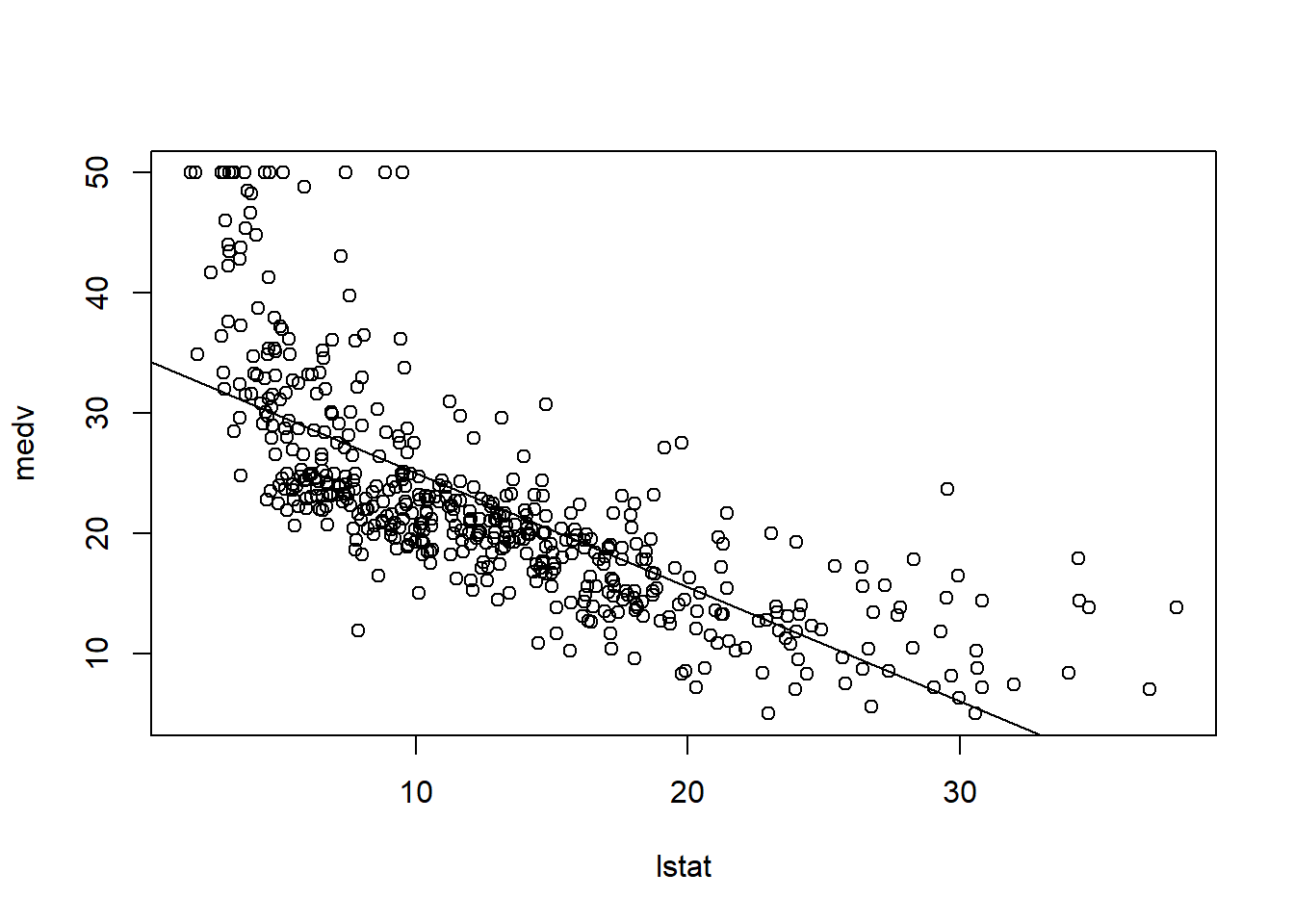

plot(lstat ,medv ,col ="red ")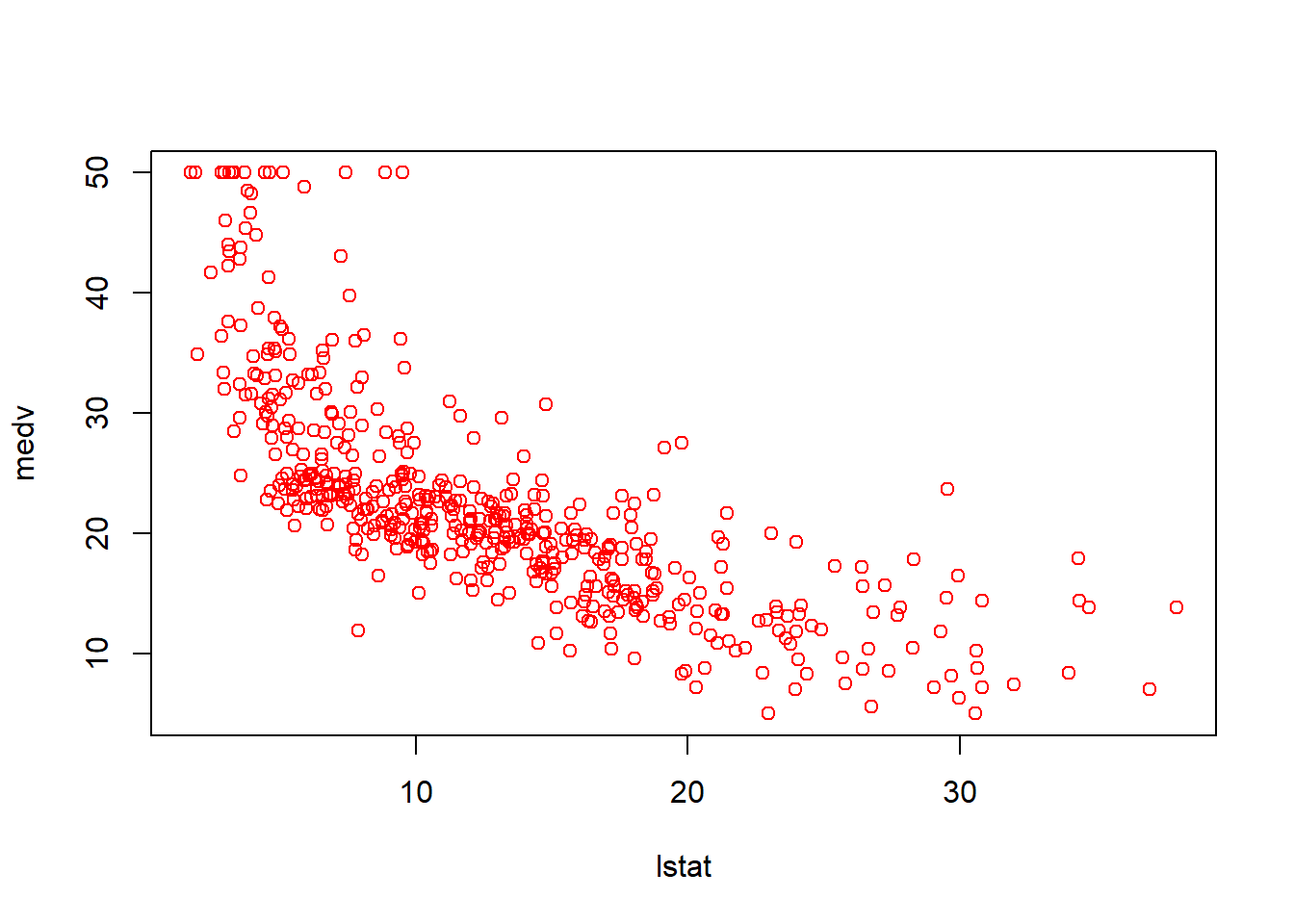

plot(lstat ,medv ,pch =20)

plot(lstat ,medv ,pch ="+")

plot (1:20 ,1:20, pch =1:20)
abline (lm.fit ,lwd =3)
abline (lm.fit ,lwd =3, col ="red ")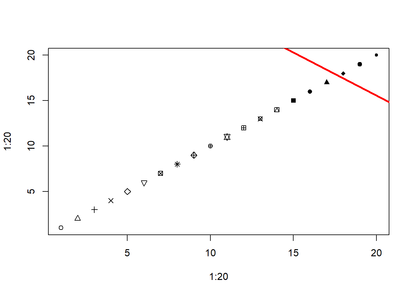

par(mfrow =c(2,2))
plot(lm.fit)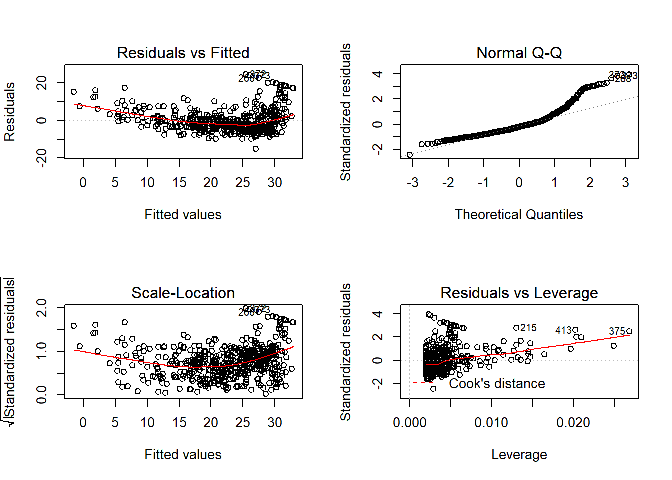

plot(predict (lm.fit), residuals (lm.fit))

plot(predict (lm.fit), rstudent (lm.fit))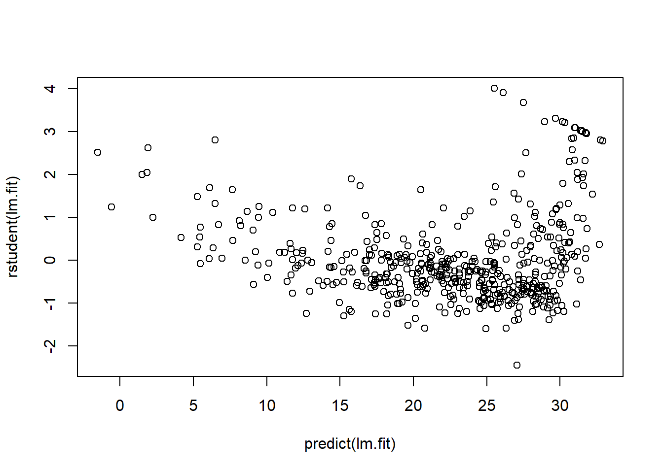

plot(hatvalues(lm.fit ))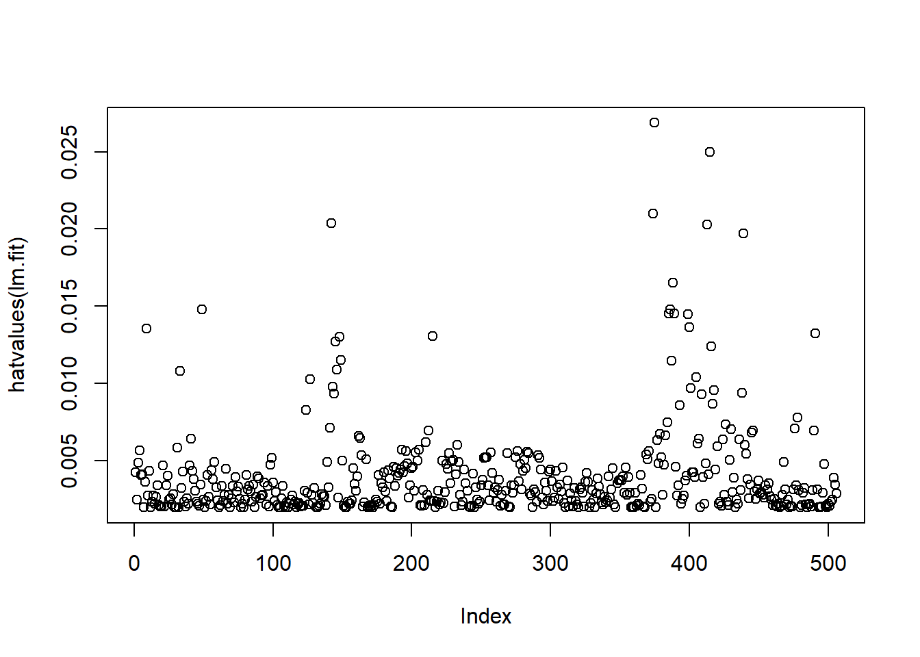

which.max (hatvalues(lm.fit))
## 375 
## 375