By Salerno | October 8, 2022
1) Introduction
What about knowing more about some important concepts around manipulating data sets? We definitely know how it is tough working in the real problems world, a lot of information sprawled in many databases.
With the knowledge shared below you’ll probably find a solution that fits in your day-a-day as data scientists.
Enjoy my folks!
2) Datasets
parts <- readRDS('C://Users//andre//OneDrive//Documentos//Private//Salerno//Pessoal//Cursos//datacamp//dplyr//parts.rds')

parts_categories <- readRDS('C://Users//andre//OneDrive//Documentos//Private//Salerno//Pessoal//Cursos//datacamp//dplyr//part_categories.rds')

inventories <- readRDS('C://Users//andre//OneDrive//Documentos//Private//Salerno//Pessoal//Cursos//datacamp//dplyr//inventories.rds')

inventory_parts <- readRDS('C://Users//andre//OneDrive//Documentos//Private//Salerno//Pessoal//Cursos//datacamp//dplyr//inventory_parts.rds')

sets <- readRDS('C://Users//andre//OneDrive//Documentos//Private//Salerno//Pessoal//Cursos//datacamp//dplyr//sets.rds')

colors <- readRDS('C://Users//andre//OneDrive//Documentos//Private//Salerno//Pessoal//Cursos//datacamp//dplyr//colors.rds')

themes <- readRDS('C://Users//andre//OneDrive//Documentos//Private//Salerno//Pessoal//Cursos//datacamp//dplyr//themes.rds')

color_palette <- readxl::read_xlsx("C://Users//andre//OneDrive//Documentos//Private//Salerno//Pessoal//Cursos//datacamp//dplyr//color_palette.xlsx")

questions <- readRDS("C://Users//andre//OneDrive//Documentos//Private//Salerno//Pessoal//Cursos//datacamp//dplyr//questions.rds")

question_tags <- readRDS("C://Users//andre//OneDrive//Documentos//Private//Salerno//Pessoal//Cursos//datacamp//dplyr//question_tags.rds")

tags <- readRDS("C://Users//andre//OneDrive//Documentos//Private//Salerno//Pessoal//Cursos//datacamp//dplyr//tags.rds")

answers <- readRDS("C://Users//andre//OneDrive//Documentos//Private//Salerno//Pessoal//Cursos//datacamp//dplyr//answers.rds")
3) Knowing dimensionals
dim(parts)
## [1] 17501     3
colnames(parts)
## [1] "part_num"    "name"        "part_cat_id"

dim(parts_categories)
## [1] 64  2
colnames(parts_categories)
## [1] "id"   "name"

dim(inventories)
## [1] 15174     3
colnames(inventories)
## [1] "id"      "version" "set_num"

dim(inventory_parts)
## [1] 258958      4
colnames(inventory_parts)
## [1] "inventory_id" "part_num"     "color_id"     "quantity"

dim(sets)
## [1] 4977    4
colnames(sets)
## [1] "set_num"  "name"     "year"     "theme_id"

dim(colors)
## [1] 179   3
colnames(colors)
## [1] "id"   "name" "rgb"
4) Joining parts and part categories
So, in this stage we’ve decided to create a new object called parts_join as a result of the use of parts dataset and parts_categories, unified by columns named part_cat_id (first dataset) and id (second dataset) respectively.
As mention above, before joining we have 3 columns by the parts data set, and parts_catogories has 2 columns.
As a result of this joining process, we’ll have 3 columns that were unified by the attributes part_cat_id from the parts and id from the parts_categories dataset.
parts %>%
  count(part_cat_id, sort = TRUE)
## # A tibble: 63 × 2
##    part_cat_id     n
##          <dbl> <int>
##  1          60  2091
##  2           4  1900
##  3          59  1565
##  4          27   937
##  5          61   805
##  6          19   804
##  7          65   803
##  8          41   701
##  9          28   529
## 10          58   518
## # … with 53 more rows
parts_categories %>%
  count(id, sort = TRUE)
## # A tibble: 64 × 2
##       id     n
##    <dbl> <int>
##  1     1     1
##  2     3     1
##  3     4     1
##  4     5     1
##  5     6     1
##  6     7     1
##  7     8     1
##  8     9     1
##  9    11     1
## 10    12     1
## # … with 54 more rows
There is an important verb called inner join. Check out the image below:
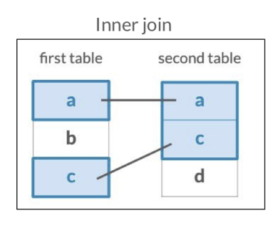 We obtain a new table where the attributes in the first table is incremented with the columns with the second table.
parts_join <- parts %>%
      inner_join(parts_categories, by = c("part_cat_id" = "id"), suffix = c("_part", "_category"))

head(parts_join)
## # A tibble: 6 × 4
##   part_num name_part                                   part_cat_id name_category
##   <chr>    <chr>                                             <dbl> <chr>
## 1 0901     Baseplate 16 x 30 with Set 080 Yellow Hous…           1 Baseplates
## 2 0902     Baseplate 16 x 24 with Set 080 Small White…           1 Baseplates
## 3 0903     Baseplate 16 x 24 with Set 080 Red House P…           1 Baseplates
## 4 0904     Baseplate 16 x 24 with Set 080 Large White…           1 Baseplates
## 5 1        Homemaker Bookcase 2 x 4 x 4                          7 Containers
## 6 10016414 Sticker Sheet #1 for 41055-1                         58 Stickers

colnames(parts_join)
## [1] "part_num"      "name_part"     "part_cat_id"   "name_category"
colnames(parts)
## [1] "part_num"    "name"        "part_cat_id"
parts %>%
  count(part_num)
## # A tibble: 17,501 × 2
##    part_num       n
##    <chr>      <int>
##  1 0901           1
##  2 0902           1
##  3 0903           1
##  4 0904           1
##  5 1              1
##  6 10016414       1
##  7 10026stk01     1
##  8 10039          1
##  9 10048          1
## 10 10049          1
## # … with 17,491 more rows

colnames(inventory_parts)
## [1] "inventory_id" "part_num"     "color_id"     "quantity"
inventory_parts %>%
  count(part_num)
## # A tibble: 17,501 × 2
##    part_num       n
##    <chr>      <int>
##  1 0901           1
##  2 0902           1
##  3 0903           1
##  4 0904           1
##  5 1              7
##  6 10016414       1
##  7 10026stk01     1
##  8 10039          4
##  9 10048          3
## 10 10049          2
## # … with 17,491 more rows

parts %>%
  inner_join(inventory_parts, by = c("part_num" = "part_num"))
## # A tibble: 258,958 × 6
##    part_num name                      part_cat_id inventory_id color_id quantity
##    <chr>    <chr>                           <dbl>        <dbl>    <dbl>    <dbl>
##  1 0901     Baseplate 16 x 30 with S…           1         1973        2        1
##  2 0902     Baseplate 16 x 24 with S…           1         1973        2        1
##  3 0903     Baseplate 16 x 24 with S…           1         1973        2        1
##  4 0904     Baseplate 16 x 24 with S…           1         1973        2        1
##  5 1        Homemaker Bookcase 2 x 4…           7          508       15        1
##  6 1        Homemaker Bookcase 2 x 4…           7         1158       15        2
##  7 1        Homemaker Bookcase 2 x 4…           7         6590       15        2
##  8 1        Homemaker Bookcase 2 x 4…           7         9679       15        2
##  9 1        Homemaker Bookcase 2 x 4…           7        12256        1        2
## 10 1        Homemaker Bookcase 2 x 4…           7        13356       15        1
## # … with 258,948 more rows
5) Joining two tables
sets %>%
  # Add inventories using an inner join
  inner_join(inventories, by = c('set_num' = 'set_num' )) %>%
  # Add inventory_parts using an inner join
  inner_join(inventory_parts, by = c('id' = 'inventory_id'))
## # A tibble: 258,958 × 9
##    set_num name           year theme_id    id version part_num color_id quantity
##    <chr>   <chr>         <dbl>    <dbl> <dbl>   <dbl> <chr>       <dbl>    <dbl>
##  1 700.3-1 Medium Gift …  1949      365 24197       1 bdoor01         2        2
##  2 700.3-1 Medium Gift …  1949      365 24197       1 bdoor01        15        1
##  3 700.3-1 Medium Gift …  1949      365 24197       1 bdoor01         4        1
##  4 700.3-1 Medium Gift …  1949      365 24197       1 bslot02        15        6
##  5 700.3-1 Medium Gift …  1949      365 24197       1 bslot02         2        6
##  6 700.3-1 Medium Gift …  1949      365 24197       1 bslot02         4        6
##  7 700.3-1 Medium Gift …  1949      365 24197       1 bslot02         1        6
##  8 700.3-1 Medium Gift …  1949      365 24197       1 bslot02        14        6
##  9 700.3-1 Medium Gift …  1949      365 24197       1 bslot02a       15        6
## 10 700.3-1 Medium Gift …  1949      365 24197       1 bslot02a        2        6
## # … with 258,948 more rows
colnames(sets)
## [1] "set_num"  "name"     "year"     "theme_id"
colnames(inventories)
## [1] "id"      "version" "set_num"
colnames(inventory_parts)
## [1] "inventory_id" "part_num"     "color_id"     "quantity"
colnames(colors)
## [1] "id"   "name" "rgb"
6) Joining three tables
# Add an inner join for the colors table
sets %>%
  inner_join(inventories, by = "set_num") %>%
  inner_join(inventory_parts, by = c("id" = "inventory_id")) %>%
  inner_join(colors, by = c("color_id" = "id"), suffix = c("_set", "_color"))
## # A tibble: 258,958 × 11
##    set_num name_set       year theme_id    id version part_num color_id quantity
##    <chr>   <chr>         <dbl>    <dbl> <dbl>   <dbl> <chr>       <dbl>    <dbl>
##  1 700.3-1 Medium Gift …  1949      365 24197       1 bdoor01         2        2
##  2 700.3-1 Medium Gift …  1949      365 24197       1 bdoor01        15        1
##  3 700.3-1 Medium Gift …  1949      365 24197       1 bdoor01         4        1
##  4 700.3-1 Medium Gift …  1949      365 24197       1 bslot02        15        6
##  5 700.3-1 Medium Gift …  1949      365 24197       1 bslot02         2        6
##  6 700.3-1 Medium Gift …  1949      365 24197       1 bslot02         4        6
##  7 700.3-1 Medium Gift …  1949      365 24197       1 bslot02         1        6
##  8 700.3-1 Medium Gift …  1949      365 24197       1 bslot02        14        6
##  9 700.3-1 Medium Gift …  1949      365 24197       1 bslot02a       15        6
## 10 700.3-1 Medium Gift …  1949      365 24197       1 bslot02a        2        6
## # … with 258,948 more rows, and 2 more variables: name_color <chr>, rgb <chr>
# Count the number of colors and sort
sets %>%
  inner_join(inventories, by = "set_num") %>%
  inner_join(inventory_parts, by = c("id" = "inventory_id")) %>%
  inner_join(colors, by = c("color_id" = "id"), suffix = c("_set", "_color")) %>%
  count(name_color, sort = TRUE)
## # A tibble: 134 × 2
##    name_color            n
##    <chr>             <int>
##  1 Black             48068
##  2 White             30105
##  3 Light Bluish Gray 26024
##  4 Red               21602
##  5 Dark Bluish Gray  19948
##  6 Yellow            17088
##  7 Blue              12980
##  8 Light Gray         8632
##  9 Reddish Brown      6960
## 10 Tan                6664
## # … with 124 more rows
inventory_parts_joined <- inventories %>%
  inner_join(inventory_parts, by = c("id" = "inventory_id")) %>%
  select(-id, -version) %>%
  arrange(desc(quantity))

inventory_parts_joined
## # A tibble: 258,958 × 4
##    set_num  part_num color_id quantity
##    <chr>    <chr>       <dbl>    <dbl>
##  1 40179-1  3024           72      900
##  2 40179-1  3024           15      900
##  3 40179-1  3024            0      900
##  4 40179-1  3024           71      900
##  5 40179-1  3024           14      900
##  6 k34434-1 3024           15      810
##  7 21010-1  3023          320      771
##  8 k34431-1 3024            0      720
##  9 42083-1  2780            0      684
## 10 k34434-1 3024            0      540
## # … with 258,948 more rows
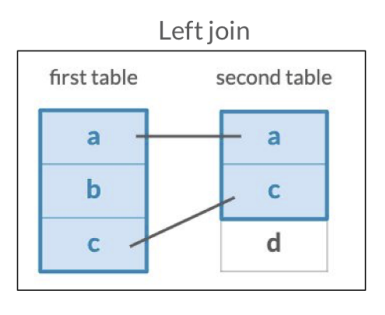
7) Left joining two sets by part and color
According with the image below, the left join function maintain all the rows in the table on the left, while increment some attributes matched in the second table.
batmobile <- inventory_parts_joined %>%
  filter(set_num == "7784-1") %>%
  select(-set_num)
batwing <- inventory_parts_joined %>%
  filter(set_num == "70916-1") %>%
  select(-set_num)
batmobile %>%
  inner_join(batwing, by = c("part_num", "color_id"), suffix = c("_batmobile", "_batwing"))
## # A tibble: 45 × 4
##    part_num color_id quantity_batmobile quantity_batwing
##    <chr>       <dbl>              <dbl>            <dbl>
##  1 2780            0                 28               17
##  2 50950           0                 28                2
##  3 3004           71                 26                2
##  4 43093           1                 25                6
##  5 3004            0                 23                4
##  6 3622            0                 18                2
##  7 4286            0                 16                1
##  8 3039            0                 12                2
##  9 4274           71                 12                7
## 10 3001            0                 11                4
## # … with 35 more rows
batmobile %>%
  left_join(batwing, by =c("part_num","color_id"), suffix =c("_batmobile","_batwing"))
## # A tibble: 173 × 4
##    part_num color_id quantity_batmobile quantity_batwing
##    <chr>       <dbl>              <dbl>            <dbl>
##  1 3023           72                 62               NA
##  2 2780            0                 28               17
##  3 50950           0                 28                2
##  4 3004           71                 26                2
##  5 43093           1                 25                6
##  6 3004            0                 23                4
##  7 3010            0                 21               NA
##  8 30363           0                 21               NA
##  9 32123b         14                 19               NA
## 10 3622            0                 18                2
## # … with 163 more rows
millennium_falcon <- inventory_parts_joined %>%
  filter(set_num == "7965-1")

star_destroyer <- inventory_parts_joined %>%
  filter(set_num == "75190-1")
# Combine the star_destroyer and millennium_falcon tables
millennium_falcon %>%
  left_join(star_destroyer, by = c("part_num", "color_id"), suffix = c("_falcon", "_star_destroyer"))
## # A tibble: 263 × 6
##    set_num_falcon part_num color_id quantity_falcon set_num_star_destroyer
##    <chr>          <chr>       <dbl>           <dbl> <chr>
##  1 7965-1         63868          71              62 <NA>
##  2 7965-1         3023            0              60 <NA>
##  3 7965-1         3021           72              46 75190-1
##  4 7965-1         2780            0              37 75190-1
##  5 7965-1         60478          72              36 <NA>
##  6 7965-1         6636           71              34 75190-1
##  7 7965-1         3009           71              28 75190-1
##  8 7965-1         3665           71              22 <NA>
##  9 7965-1         2412b          72              20 75190-1
## 10 7965-1         3010           71              19 <NA>
## # … with 253 more rows, and 1 more variable: quantity_star_destroyer <dbl>
8) Left joining two sets by color
# Aggregate Millennium Falcon for the total quantity in each part
millennium_falcon_colors <- millennium_falcon %>%
  group_by(color_id) %>%
  summarize(total_quantity = sum(quantity))

# Aggregate Star Destroyer for the total quantity in each part
star_destroyer_colors <- star_destroyer %>%
  group_by(color_id) %>%
  summarize(total_quantity = sum(quantity))

# Left join the Millennium Falcon colors to the Star Destroyer colors
millennium_falcon_colors %>%
  left_join(star_destroyer_colors, by = c("color_id"), suffix = c("_falcon", "_star_destroyer"))
## # A tibble: 21 × 3
##    color_id total_quantity_falcon total_quantity_star_destroyer
##       <dbl>                 <dbl>                         <dbl>
##  1        0                   201                           336
##  2        1                    15                            23
##  3        4                    17                            53
##  4       14                     3                             4
##  5       15                    15                            17
##  6       19                    95                            12
##  7       28                     3                            16
##  8       33                     5                            NA
##  9       36                     1                            14
## 10       41                     6                            15
## # … with 11 more rows
inventory_version_1 <- inventories %>%
  filter(version == 1)

# Join versions to sets
sets %>%
  left_join(inventory_version_1, by = "set_num") %>%
  # Filter for where version is na
  filter(is.na(version))
## # A tibble: 1 × 6
##   set_num name       year theme_id    id version
##   <chr>   <chr>     <dbl>    <dbl> <dbl>   <dbl>
## 1 40198-1 Ludo game  2018      598    NA      NA
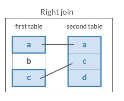
9) Counting part colors
In this chapter, we introduce the right join verb, which describes the match between two tables, and the result in concentrate on the right table. Check the image out below:
parts %>%
  # Count the part_cat_id
  count(part_cat_id) %>%
  # Right join part_categories
  right_join(parts_categories, by = c("part_cat_id" = "id")) %>%
  filter(is.na(n))
## # A tibble: 1 × 3
##   part_cat_id     n name
##         <dbl> <int> <chr>
## 1          66    NA Modulex
parts %>%
  count(part_cat_id) %>%
  right_join(parts_categories, by = c("part_cat_id" = "id")) %>%
  # Use replace_na to replace missing values in the n column
  tidyr::replace_na(list(n = 0))
## # A tibble: 64 × 3
##    part_cat_id     n name
##          <dbl> <int> <chr>
##  1           1   135 Baseplates
##  2           3   303 Bricks Sloped
##  3           4  1900 Duplo, Quatro and Primo
##  4           5   107 Bricks Special
##  5           6   128 Bricks Wedged
##  6           7    97 Containers
##  7           8    24 Technic Bricks
##  8           9   167 Plates Special
##  9          11   490 Bricks
## 10          12    85 Technic Connectors
## # … with 54 more rows
10) Joining themes to their children
themes %>%
  # Inner join the themes table
  inner_join(themes, by = c("id" = "parent_id"), suffix = c("_parent", "_child")) %>%
  # Filter for the "Harry Potter" parent name
  filter(name_parent == "Harry Potter")
## # A tibble: 6 × 5
##      id name_parent  parent_id id_child name_child
##   <dbl> <chr>            <dbl>    <dbl> <chr>
## 1   246 Harry Potter        NA      247 Chamber of Secrets
## 2   246 Harry Potter        NA      248 Goblet of Fire
## 3   246 Harry Potter        NA      249 Order of the Phoenix
## 4   246 Harry Potter        NA      250 Prisoner of Azkaban
## 5   246 Harry Potter        NA      251 Sorcerer's Stone
## 6   246 Harry Potter        NA      667 Fantastic Beasts
11) Joining themes to their grandchildren
# Join themes to itself again to find the grandchild relationships
themes %>%
  inner_join(themes, by = c("id" = "parent_id"), suffix = c("_parent", "_child")) %>%
  inner_join(themes, by = c("id_child" = "parent_id"), suffix = c("_parent", "_grandchild"))
## # A tibble: 158 × 7
##    id_parent name_parent parent_id id_child name_child id_grandchild name
##        <dbl> <chr>           <dbl>    <dbl> <chr>              <dbl> <chr>
##  1         1 Technic            NA        5 Model                  6 Airport
##  2         1 Technic            NA        5 Model                  7 Constructi…
##  3         1 Technic            NA        5 Model                  8 Farm
##  4         1 Technic            NA        5 Model                  9 Fire
##  5         1 Technic            NA        5 Model                 10 Harbor
##  6         1 Technic            NA        5 Model                 11 Off-Road
##  7         1 Technic            NA        5 Model                 12 Race
##  8         1 Technic            NA        5 Model                 13 Riding Cyc…
##  9         1 Technic            NA        5 Model                 14 Robot
## 10         1 Technic            NA        5 Model                 15 Traffic
## # … with 148 more rows
12) Left joining a table to itself
themes %>%
  # Left join the themes table to its own children
  left_join(themes, by = c("id" = "parent_id"), suffix = c("_parent", "_child")) %>%
  # Filter for themes that have no child themes
  filter(is.na(name_child))
## # A tibble: 586 × 5
##       id name_parent    parent_id id_child name_child
##    <dbl> <chr>              <dbl>    <dbl> <chr>
##  1     2 Arctic Technic         1       NA <NA>
##  2     3 Competition            1       NA <NA>
##  3     4 Expert Builder         1       NA <NA>
##  4     6 Airport                5       NA <NA>
##  5     7 Construction           5       NA <NA>
##  6     8 Farm                   5       NA <NA>
##  7     9 Fire                   5       NA <NA>
##  8    10 Harbor                 5       NA <NA>
##  9    11 Off-Road               5       NA <NA>
## 10    12 Race                   5       NA <NA>
## # … with 576 more rows
13) Differences between Batman and Star Wars
dim(inventory_parts_joined)
## [1] 258958      4

# Start with inventory_parts_joined table
inventory_sets_themes <- inventory_parts_joined %>%
      # Combine with the sets table
      inner_join(sets, by = "set_num") %>%
      # Combine with the themes table
      inner_join(themes, by = c("theme_id" = "id"), suffix = c("_set", "_theme"))

dim(inventory_sets_themes)
## [1] 258958      9
14) Aggregating each theme
batman <- inventory_sets_themes %>%
  filter(name_theme == "Batman")
star_wars <- inventory_sets_themes %>%
  filter(name_theme == "Star Wars")
# Count the part number and color id, weight by quantity
batman_parts <- batman %>%
  count(part_num, color_id, wt = quantity)

star_wars_parts <- star_wars %>%
  count(part_num, color_id, wt = quantity)
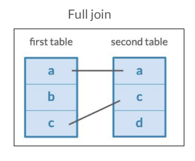
15) Full joining Batman and Star Wars LEGO parts
The full join aggregates the rows from the two tables (left and join) even though than does not have any match.
parts_joined <- batman_parts %>%
  # Combine the star_wars_parts table
  full_join(star_wars_parts, by = c("part_num", "color_id"), suffix = c("_batman", "_star_wars")) %>%
  # Replace NAs with 0s in the n_batman and n_star_wars columns
  tidyr::replace_na(list(n_batman = 0,
                  n_star_wars = 0))
16) Comparing Batman and Star Wars LEGO parts
parts_joined %>%
  # Sort the number of star wars pieces in descending order
  arrange(desc(n_star_wars)) %>%
  # Join the colors table to the parts_joined table
  inner_join(colors, by = c("color_id" = "id")) %>%
  # Join the parts table to the previous join
  inner_join(parts, by = "part_num", suffix = c("_color", "_part"))
## # A tibble: 3,628 × 8
##    part_num color_id n_batman n_star_wars name_color rgb   name_part part_cat_id
##    <chr>       <dbl>    <dbl>       <dbl> <chr>      <chr> <chr>           <dbl>
##  1 2780            0      104         392 Black      #051… Technic …          53
##  2 32062           0        1         141 Black      #051… Technic …          46
##  3 4274            1       56         118 Blue       #005… Technic …          53
##  4 6141           36       11         117 Trans-Red  #C91… Plate Ro…          21
##  5 3023           71       10         106 Light Blu… #A0A… Plate 1 …          14
##  6 6558            1       30         106 Blue       #005… Technic …          53
##  7 43093           1       44          99 Blue       #005… Technic …          53
##  8 3022           72       14          95 Dark Blui… #6C6… Plate 2 …          14
##  9 2357           19        0          84 Tan        #E4C… Brick 2 …          11
## 10 6141          179       90          81 Flat Silv… #898… Plate Ro…          21
## # … with 3,618 more rows
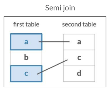
17) Something within one set but not another
With the semi join verb it aggregates only when you find match between left and right tables.
# Filter the batwing set for parts that are also in the batmobile set
batwing %>%
  semi_join(batmobile, by = c("part_num"))
## # A tibble: 126 × 3
##    part_num color_id quantity
##    <chr>       <dbl>    <dbl>
##  1 3023            0       22
##  2 3024            0       22
##  3 3623            0       20
##  4 2780            0       17
##  5 3666            0       16
##  6 3710            0       14
##  7 6141            4       12
##  8 2412b          71       10
##  9 6141           72       10
## 10 6558            1        9
## # … with 116 more rows

# Filter the batwing set for parts that aren't in the batmobile set
batwing %>%
  anti_join(batmobile, by = c("part_num"))
## # A tibble: 183 × 3
##    part_num color_id quantity
##    <chr>       <dbl>    <dbl>
##  1 11477           0       18
##  2 99207          71       18
##  3 22385           0       14
##  4 99563           0       13
##  5 10247          72       12
##  6 2877           72       12
##  7 61409          72       12
##  8 11153           0       10
##  9 98138          46       10
## 10 2419           72        9
## # … with 173 more rows
18) What colors are included in at least one set?
# Use inventory_parts to find colors included in at least one set
colors %>%
  semi_join(inventory_parts, by = c("id" = "color_id"))
## # A tibble: 134 × 3
##       id name           rgb
##    <dbl> <chr>          <chr>
##  1    -1 [Unknown]      #0033B2
##  2     0 Black          #05131D
##  3     1 Blue           #0055BF
##  4     2 Green          #237841
##  5     3 Dark Turquoise #008F9B
##  6     4 Red            #C91A09
##  7     5 Dark Pink      #C870A0
##  8     6 Brown          #583927
##  9     7 Light Gray     #9BA19D
## 10     8 Dark Gray      #6D6E5C
## # … with 124 more rows
19) Which set is missing version 1?
# Use filter() to extract version 1
version_1_inventories <- inventories %>%
  filter(version == 1)

# Use anti_join() to find which set is missing a version 1
sets %>%
  anti_join(version_1_inventories, by = c("set_num" = "set_num"))
## # A tibble: 1 × 4
##   set_num name       year theme_id
##   <chr>   <chr>     <dbl>    <dbl>
## 1 40198-1 Ludo game  2018      598
20) Aggregating sets to look at their differences
inventory_parts_themes <- inventories %>%
  inner_join(inventory_parts, by = c("id" = "inventory_id")) %>%
  arrange(desc(quantity)) %>%
  select(-id, -version) %>%
  inner_join(sets, by = "set_num") %>%
  inner_join(themes, by = c("theme_id" = "id"), suffix = c("_set", "_theme"))

batman_colors <- inventory_parts_themes %>%
  # Filter the inventory_parts_themes table for the Batman theme
  filter(name_theme == "Batman") %>%
  group_by(color_id) %>%
  summarize(total = sum(quantity)) %>%
  # Add a fraction column of the total divided by the sum of the total
  mutate(fraction = total / sum(total))

# Filter and aggregate the Star Wars set data; add a fraction column
star_wars_colors <- inventory_parts_themes %>%
  filter(name_theme == "Star Wars") %>%
  group_by(color_id) %>%
  summarize(total = sum(quantity)) %>%
  # Add a fraction column of the total divided by the sum of the total
  mutate(fraction = total / sum(total))
21) Combining sets
batman_colors %>%
  full_join(star_wars_colors, by = "color_id", suffix = c("_batman", "_star_wars")) %>%
  tidyr::replace_na(list(total_batman = 0, total_star_wars = 0)) %>%
  inner_join(colors, by = c("color_id" = "id")) %>%
  # Create the difference and total columns
  mutate(difference = fraction_batman - fraction_star_wars,
         total = total_batman + total_star_wars) %>%
  # Filter for totals greater than 200
  filter(total > 200) %>%
  arrange(desc(difference))
## # A tibble: 16 × 9
##    color_id total_batman fraction_batman total_star_wars fraction_star_wa… name
##       <dbl>        <dbl>           <dbl>           <dbl>             <dbl> <chr>
##  1        0         2807         0.296              3258           0.207   Black
##  2       14          426         0.0449              207           0.0132  Yell…
##  3        4          529         0.0558              434           0.0276  Red
##  4       84          278         0.0293               31           0.00197 Medi…
##  5       46          200         0.0211               39           0.00248 Tran…
##  6       70          297         0.0313              373           0.0237  Redd…
##  7      179          154         0.0162              232           0.0148  Flat…
##  8        1          243         0.0256              410           0.0261  Blue
##  9       28           98         0.0103              183           0.0116  Dark…
## 10       72         1453         0.153              2433           0.155   Dark…
## 11       36           86         0.00907             246           0.0156  Tran…
## 12      378           22         0.00232             430           0.0273  Sand…
## 13       19          142         0.0150             1012           0.0644  Tan
## 14       15          404         0.0426             1771           0.113   White
## 15       71         1148         0.121              3264           0.208   Ligh…
## 16        7            0        NA                   209           0.0133  Ligh…
## # … with 3 more variables: rgb <chr>, difference <dbl>, total <dbl>
22) Visualizing the difference: Batman and Star Wars
library(forcats)
## Warning: package 'forcats' was built under R version 4.2.1

colors_joined <- batman_colors %>%
  full_join(star_wars_colors, by = "color_id", suffix = c("_batman", "_star_wars")) %>%
  tidyr::replace_na(list(total_batman = 0, total_star_wars = 0)) %>%
  inner_join(colors, by = c("color_id" = "id")) %>%
  mutate(difference = fraction_batman - fraction_star_wars,
         total = total_batman + total_star_wars) %>%
  filter(total >= 200) %>%
  mutate(name = fct_reorder(name, difference))
library(ggplot2)
## Warning: package 'ggplot2' was built under R version 4.2.1

#color_palette_fct <- as.vector(color_palette$color_name)

color_palette<- as.vector(color_palette$id)

#color_palette <- factor(color_palette$id, levels = color_palette_fct)

# Create a bar plot using colors_joined and the name and difference columns
ggplot(colors_joined, aes(name, difference, fill = name)) +
  geom_col() +
  coord_flip() +
  scale_fill_manual(values = color_palette, guide = "none") +
  labs(y = "Difference: Batman - Star Wars")
## Warning: Removed 1 rows containing missing values (position_stack).
# Replace the NAs in the tag_name column
questions_with_tags <- questions %>%
  left_join(question_tags, by = c("id" = "question_id")) %>%
  left_join(tags, by = c("tag_id" = "id")) %>%
  tidyr::replace_na(list(tag_name = "only-r"))
24) Comparing scores across tags
questions_with_tags %>%
  # Group by tag_name
  group_by(tag_name) %>%
  # Get mean score and num_questions
  summarize(score = mean(score),
        	num_questions = n()) %>%
  # Sort num_questions in descending order
  arrange(desc(num_questions))
## # A tibble: 7,841 × 3
##    tag_name   score num_questions
##    <chr>      <dbl>         <int>
##  1 only-r     1.26          48541
##  2 ggplot2    2.61          28228
##  3 dataframe  2.31          18874
##  4 shiny      1.45          14219
##  5 dplyr      1.95          14039
##  6 plot       2.24          11315
##  7 data.table 2.97           8809
##  8 matrix     1.66           6205
##  9 loops      0.743          5149
## 10 regex      2              4912
## # … with 7,831 more rows
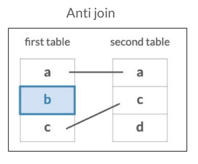
25) What tags never appear on R questions?
And if you looking for some events that does not appear in the right table? So, in this case we recommend to use anti join.
# Using a join, filter for tags that are never on an R question
tags %>%
  anti_join(question_tags, by = c("id" = "tag_id"))
## # A tibble: 40,459 × 2
##        id tag_name
##     <dbl> <chr>
##  1 124399 laravel-dusk
##  2 124402 spring-cloud-vault-config
##  3 124404 spring-vault
##  4 124405 apache-bahir
##  5 124407 astc
##  6 124408 simulacrum
##  7 124410 angulartics2
##  8 124411 django-rest-viewsets
##  9 124414 react-native-lightbox
## 10 124417 java-module
## # … with 40,449 more rows
26) Finding gaps between questions and answers
questions %>%
  # Inner join questions and answers with proper suffixes
  inner_join(answers, by = c("id" = "question_id"), suffix = c("_question", "_answer")) %>%
  # Subtract creation_date_question from creation_date_answer to create gap
  mutate(gap = as.integer(creation_date_question - creation_date_answer))
## # A tibble: 380,643 × 7
##          id creation_date_question score_question id_answer creation_date_answer
##       <int> <date>                          <int>     <int> <date>
##  1 22557677 2014-03-21                          1  22560670 2014-03-21
##  2 22557707 2014-03-21                          2  22558516 2014-03-21
##  3 22557707 2014-03-21                          2  22558726 2014-03-21
##  4 22558084 2014-03-21                          2  22558085 2014-03-21
##  5 22558084 2014-03-21                          2  22606545 2014-03-24
##  6 22558084 2014-03-21                          2  22610396 2014-03-24
##  7 22558084 2014-03-21                          2  34374729 2015-12-19
##  8 22558395 2014-03-21                          2  22559327 2014-03-21
##  9 22558395 2014-03-21                          2  22560102 2014-03-21
## 10 22558395 2014-03-21                          2  22560288 2014-03-21
## # … with 380,633 more rows, and 2 more variables: score_answer <int>, gap <int>
27) Joining question and answer counts
# Count and sort the question id column in the answers table
answer_counts <- answers %>%
  count(question_id, sort = TRUE)

# Combine the answer_counts and questions tables
questions %>%
  left_join(answer_counts, by = c("id" = "question_id")) %>%
  # Replace the NAs in the n column
  tidyr::replace_na(list(n = 0))
## # A tibble: 294,735 × 4
##          id creation_date score     n
##       <int> <date>        <int> <int>
##  1 22557677 2014-03-21        1     1
##  2 22557707 2014-03-21        2     2
##  3 22558084 2014-03-21        2     4
##  4 22558395 2014-03-21        2     3
##  5 22558613 2014-03-21        0     1
##  6 22558677 2014-03-21        2     2
##  7 22558887 2014-03-21        8     1
##  8 22559180 2014-03-21        1     1
##  9 22559312 2014-03-21        0     1
## 10 22559322 2014-03-21        2     5
## # … with 294,725 more rows
28) Joining questions, answers and tags
answer_counts <- answers %>%
    count(question_id, sort = TRUE)

question_answer_counts <- questions %>%
    left_join(answer_counts, by = c("id" = "question_id")) %>%
    tidyr::replace_na(list(n = 0))
question_answer_counts %>%
  # Join the question_tags tables
  inner_join(question_tags, by = c("id" = "question_id")) %>%
  # Join the tags table
  inner_join(tags, by = c("tag_id" = "id"))
## # A tibble: 497,153 × 6
##          id creation_date score     n tag_id tag_name
##       <int> <date>        <int> <int>  <dbl> <chr>
##  1 22557677 2014-03-21        1     1     18 regex
##  2 22557677 2014-03-21        1     1    139 string
##  3 22557677 2014-03-21        1     1  16088 time-complexity
##  4 22557677 2014-03-21        1     1   1672 backreference
##  5 22558084 2014-03-21        2     4   6419 time-series
##  6 22558084 2014-03-21        2     4  92764 panel-data
##  7 22558395 2014-03-21        2     3   5569 function
##  8 22558395 2014-03-21        2     3    134 sorting
##  9 22558395 2014-03-21        2     3   9412 vectorization
## 10 22558395 2014-03-21        2     3  18621 operator-precedence
## # … with 497,143 more rows
29) Average answers by question
tagged_answers <- question_answer_counts %>%
    inner_join(question_tags, by = c("id" = "question_id")) %>%
    inner_join(tags, by = c("tag_id" = "id"))
tagged_answers %>%
  # Aggregate by tag_name
  group_by(tag_name)  %>%
  # Summarize questions and average_answers
  summarize(questions = n(),
            average_answers = mean(n)) %>%
  # Sort the questions in descending order
  arrange(desc(questions))
## # A tibble: 7,840 × 3
##    tag_name   questions average_answers
##    <chr>          <int>           <dbl>
##  1 ggplot2        28228           1.15
##  2 dataframe      18874           1.67
##  3 shiny          14219           0.921
##  4 dplyr          14039           1.55
##  5 plot           11315           1.23
##  6 data.table      8809           1.47
##  7 matrix          6205           1.45
##  8 loops           5149           1.39
##  9 regex           4912           1.91
## 10 function        4892           1.30
## # … with 7,830 more rows
30) Joining questions and answers with tags
# Inner join the question_tags and tags tables with the questions table
questions_with_tags <- questions %>%
  inner_join(question_tags, by = c("id" = "question_id")) %>%
  inner_join(tags, by = c("tag_id" = "id"))

# Inner join the question_tags and tags tables with the answers table
answers_with_tags <- answers %>%
  inner_join(question_tags, by = "question_id") %>%
  inner_join(tags, by = c("tag_id" = "id"))
31) Binding and counting posts with tags
questions_with_tags <- questions %>%
  inner_join(question_tags, by = c("id" = "question_id")) %>%
  inner_join(tags, by = c("tag_id" = "id"))
answers_with_tags <- answers %>%
  inner_join(question_tags, by = "question_id") %>%
  inner_join(tags, by = c("tag_id" = "id"))
library(lubridate)
## Warning: package 'lubridate' was built under R version 4.2.1
##
## Attaching package: 'lubridate'
## The following objects are masked from 'package:base':
##
##     date, intersect, setdiff, union
# Combine the two tables into posts_with_tags
posts_with_tags <- bind_rows(questions_with_tags %>% mutate(type = "question"),
                              answers_with_tags %>% mutate(type = "answer"))

# Add a year column, then count by type, year, and tag_name
by_type_year_tag <- posts_with_tags %>%
  mutate(year = year(creation_date)) %>%
  count(type, year, tag_name)
32) Visualizing questions and answers in tags
library(ggplot2)
# Filter for the dplyr and ggplot2 tag names
by_type_year_tag_filtered <- by_type_year_tag %>%
  filter(tag_name %in% c("dplyr", "ggplot2"))

# Create a line plot faceted by the tag name
ggplot(by_type_year_tag_filtered, aes(year, n, color = type)) +
  geom_line() +
  facet_wrap(~ tag_name)