By Bruno Ferrari | February 7, 2020
Objetive
Train a model and use to make predictions for German Credit dataset
Data
german = read.csv(path)str(german)
## 'data.frame': 1000 obs. of 21 variables:
## $ default : int 0 1 0 0 1 0 0 0 0 1 ...
## $ account_check_status : Factor w/ 4 levels "< 0 DM",">= 200 DM / salary assignments for at least 1 year",..: 1 3 4 1 1 4 4 3 4 3 ...
## $ duration_in_month : int 6 48 12 42 24 36 24 36 12 30 ...
## $ credit_history : Factor w/ 5 levels "all credits at this bank paid back duly",..: 2 4 2 4 3 4 4 4 4 2 ...
## $ purpose : Factor w/ 10 levels "(vacation - does not exist?)",..: 5 5 1 8 3 1 8 4 5 3 ...
## $ credit_amount : int 1169 5951 2096 7882 4870 9055 2835 6948 3059 5234 ...
## $ savings : Factor w/ 5 levels ".. >= 1000 DM ",..: 5 2 2 2 2 5 4 2 1 2 ...
## $ present_emp_since : Factor w/ 5 levels ".. >= 7 years",..: 1 3 4 4 3 3 1 3 4 5 ...
## $ installment_as_income_perc: int 4 2 2 2 3 2 3 2 2 4 ...
## $ personal_status_sex : Factor w/ 4 levels "female : divorced/separated/married",..: 4 1 4 4 4 4 4 4 2 3 ...
## $ other_debtors : Factor w/ 3 levels "co-applicant",..: 3 3 3 2 3 3 3 3 3 3 ...
## $ present_res_since : int 4 2 3 4 4 4 4 2 4 2 ...
## $ property : Factor w/ 4 levels "if not A121 : building society savings agreement/ life insurance",..: 3 3 3 1 4 4 1 2 3 2 ...
## $ age : int 67 22 49 45 53 35 53 35 61 28 ...
## $ other_installment_plans : Factor w/ 3 levels "bank","none",..: 2 2 2 2 2 2 2 2 2 2 ...
## $ housing : Factor w/ 3 levels "for free","own",..: 2 2 2 1 1 1 2 3 2 2 ...
## $ credits_this_bank : int 2 1 1 1 2 1 1 1 1 2 ...
## $ job : Factor w/ 4 levels "management/ self-employed/ highly qualified employee/ officer",..: 2 2 4 2 2 4 2 1 4 1 ...
## $ people_under_maintenance : int 1 1 2 2 2 2 1 1 1 1 ...
## $ telephone : Factor w/ 2 levels "none","yes, registered under the customers name ": 2 1 1 1 1 2 1 2 1 1 ...
## $ foreign_worker : Factor w/ 2 levels "no","yes": 2 2 2 2 2 2 2 2 2 2 ...As we can see, the dataset consists of twenty variables and a thousand observation, which of 30% went into default.
Model Fitting
The model that we will use in this work will be a Regression Tree. This model will provide us some benefits, the main ones being:
1 - We will not need to assume any hypothesis about the data, which is good due to the amount of variables.
2 - We also will not need to pre-process the data, we can use the raw data to fit the model.
Loading the required packages
library("rpart")
library("rpart.plot")
library("caTools")
library("caret")
Spliting the dataset into train and test.
split = sample.split(german$default, SplitRatio = 0.75)
train = subset(german, split==TRUE)
test = subset(german, split==FALSE)
Fitting the Regression Tree
tree = rpart(default ~ account_check_status + duration_in_month + credit_history +
        purpose + credit_amount + savings + present_emp_since +
        installment_as_income_perc + personal_status_sex + other_debtors + present_res_since +
        property + age + other_installment_plans + housing +
        credits_this_bank + job + people_under_maintenance + telephone + foreign_worker, data = train, method = "class")
Generated Tree
prp(tree)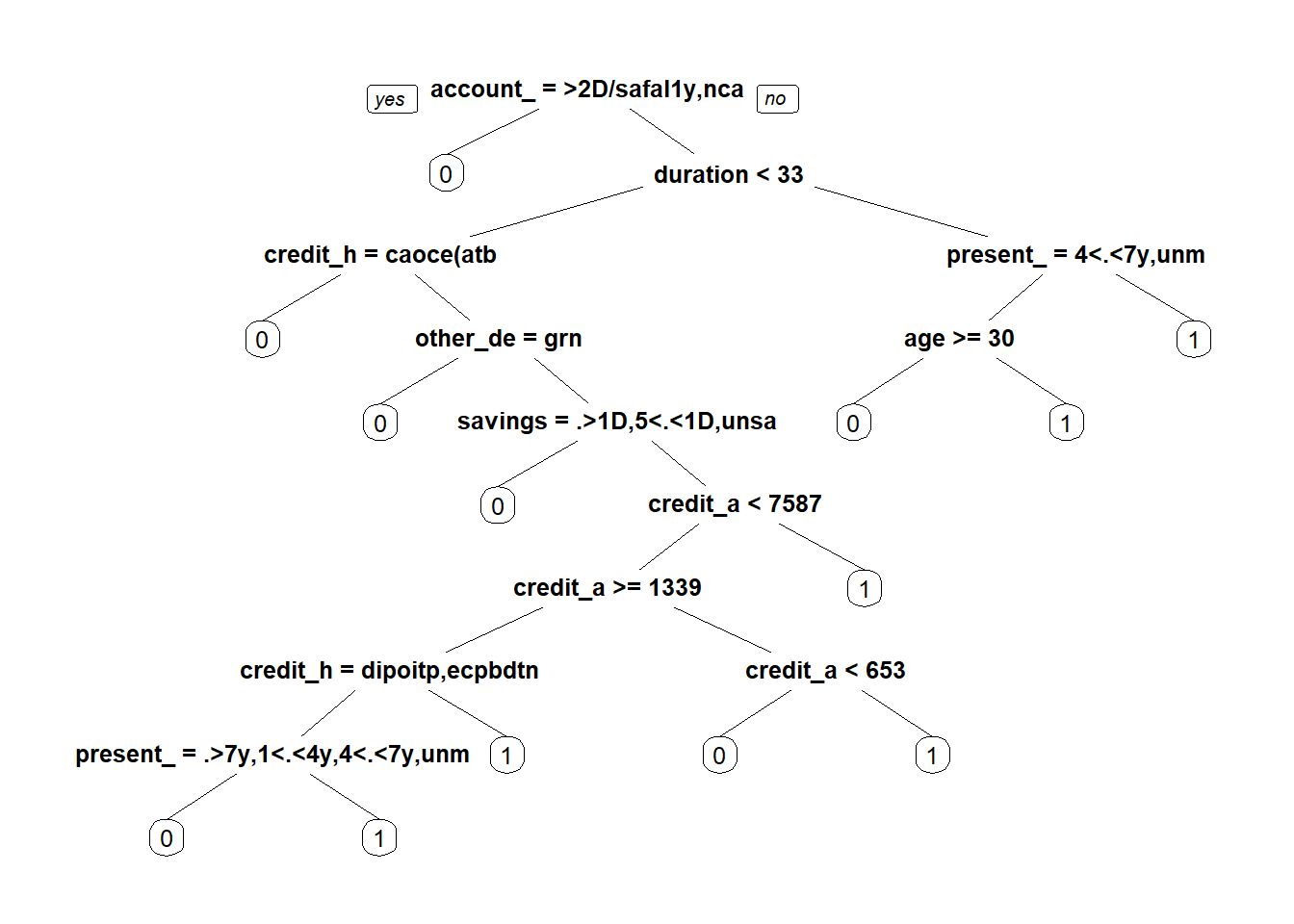
tree
## n= 750
##
## node), split, n, loss, yval, (yprob)
##       * denotes terminal node
##
##   1) root 750 225 0 (0.70000000 0.30000000)
##     2) account_check_status=>= 200 DM / salary assignments for at least 1 year,no checking account 347  48 0 (0.86167147 0.13832853) *
##     3) account_check_status=< 0 DM,0 <= ... < 200 DM 403 177 0 (0.56079404 0.43920596)
##       6) duration_in_month< 33 320 122 0 (0.61875000 0.38125000)
##        12) credit_history=critical account/ other credits existing (not at this bank) 75  15 0 (0.80000000 0.20000000) *
##        13) credit_history=all credits at this bank paid back duly,delay in paying off in the past,existing credits paid back duly till now,no credits taken/ all credits paid back duly 245 107 0 (0.56326531 0.43673469)
##          26) other_debtors=guarantor 24   2 0 (0.91666667 0.08333333) *
##          27) other_debtors=co-applicant,none 221 105 0 (0.52488688 0.47511312)
##            54) savings=.. >= 1000 DM ,500 <= ... < 1000 DM ,unknown/ no savings account 56  16 0 (0.71428571 0.28571429) *
##            55) savings=... < 100 DM,100 <= ... < 500 DM 165  76 1 (0.46060606 0.53939394)
##             110) credit_amount< 7586.5 156  76 1 (0.48717949 0.51282051)
##               220) credit_amount>=1338.5 105  45 0 (0.57142857 0.42857143)
##                 440) credit_history=delay in paying off in the past,existing credits paid back duly till now 85  31 0 (0.63529412 0.36470588)
##                   880) present_emp_since=.. >= 7 years,1 <= ... < 4 years,4 <= ... < 7 years,unemployed 67  20 0 (0.70149254 0.29850746) *
##                   881) present_emp_since=... < 1 year  18   7 1 (0.38888889 0.61111111) *
##                 441) credit_history=all credits at this bank paid back duly,no credits taken/ all credits paid back duly 20   6 1 (0.30000000 0.70000000) *
##               221) credit_amount< 1338.5 51  16 1 (0.31372549 0.68627451)
##                 442) credit_amount< 653 7   1 0 (0.85714286 0.14285714) *
##                 443) credit_amount>=653 44  10 1 (0.22727273 0.77272727) *
##             111) credit_amount>=7586.5 9   0 1 (0.00000000 1.00000000) *
##       7) duration_in_month>=33 83  28 1 (0.33734940 0.66265060)
##        14) present_emp_since=4 <= ... < 7 years,unemployed 29  13 0 (0.55172414 0.44827586)
##          28) age>=29.5 20   5 0 (0.75000000 0.25000000) *
##          29) age< 29.5 9   1 1 (0.11111111 0.88888889) *
##        15) present_emp_since=.. >= 7 years,... < 1 year ,1 <= ... < 4 years 54  12 1 (0.22222222 0.77777778) *
Confusion Matrix for train set.
fit = predict(tree, type = "class")
confusionMatrix(fit, as.factor(train$default))
## Confusion Matrix and Statistics
##
##           Reference
## Prediction   0   1
##          0 489 107
##          1  36 118
##
##                Accuracy : 0.8093
##                  95% CI : (0.7794, 0.8369)
##     No Information Rate : 0.7
##     P-Value [Acc > NIR] : 6.302e-12
##
##                   Kappa : 0.501
##
##  Mcnemar's Test P-Value : 4.808e-09
##
##             Sensitivity : 0.9314
##             Specificity : 0.5244
##          Pos Pred Value : 0.8205
##          Neg Pred Value : 0.7662
##              Prevalence : 0.7000
##          Detection Rate : 0.6520
##    Detection Prevalence : 0.7947
##       Balanced Accuracy : 0.7279
##
##        'Positive' Class : 0
##
Confusion Matrix for test set.
fit_test = predict(tree, type = "class", newdata = test[,-1])
confusionMatrix(fit_test, as.factor(test$default))
## Confusion Matrix and Statistics
##
##           Reference
## Prediction   0   1
##          0 150  42
##          1  25  33
##
##                Accuracy : 0.732
##                  95% CI : (0.6725, 0.7859)
##     No Information Rate : 0.7
##     P-Value [Acc > NIR] : 0.15012
##
##                   Kappa : 0.3177
##
##  Mcnemar's Test P-Value : 0.05062
##
##             Sensitivity : 0.8571
##             Specificity : 0.4400
##          Pos Pred Value : 0.7812
##          Neg Pred Value : 0.5690
##              Prevalence : 0.7000
##          Detection Rate : 0.6000
##    Detection Prevalence : 0.7680
##       Balanced Accuracy : 0.6486
##
##        'Positive' Class : 0
##
We can see that the accuracy of train set is a bit far from the test set. This is not a favorable scenario for the model, as it indicates a possible overfitted model, but as long as the model baseline (percentage of the greater class) is 70% of accurate, this regression tree is much better than the baseline model.
We could tune the model making some adjustment on the hyperparameters, like give a extra cost for example to False Positve cases.
False Positive, means they won’t pay the loan (default = 1), but the model thinks they will. (predicted = 0)
False Negative, means they will pay the loan (default = 0), but the model said they won’t. (predicted = 1)
Generally, the False Positive error in this case is worse, so lets make some example with a cost on that error.
cost_matrix = matrix(c(0,2,1,0), nrow=2, ncol = 2)
cost_matrix
##      [,1] [,2]
## [1,]    0    1
## [2,]    2    0
tree_p = rpart(default ~ account_check_status + duration_in_month + credit_history +
purpose + credit_amount + savings + present_emp_since +
installment_as_income_perc + personal_status_sex + other_debtors + present_res_since +
property + age + other_installment_plans + housing +
credits_this_bank + job + people_under_maintenance + telephone + foreign_worker, data = train, method = "class",
parms = list(loss = cost_matrix))fit = predict(tree_p, type = "class")
confusionMatrix(fit, as.factor(train$default))
## Confusion Matrix and Statistics
##
## Reference
## Prediction 0 1
## 0 417 43
## 1 108 182
##
## Accuracy : 0.7987
## 95% CI : (0.7682, 0.8268)
## No Information Rate : 0.7
## P-Value [Acc > NIR] : 6.141e-10
##
## Kappa : 0.5572
##
## Mcnemar's Test P-Value : 1.906e-07
##
## Sensitivity : 0.7943
## Specificity : 0.8089
## Pos Pred Value : 0.9065
## Neg Pred Value : 0.6276
## Prevalence : 0.7000
## Detection Rate : 0.5560
## Detection Prevalence : 0.6133
## Balanced Accuracy : 0.8016
##
## 'Positive' Class : 0
## In other hand, we could remove some varibles, e.g. telephone, or reduce dimensionality of the problem, like applying a PCA. In the case o PCA, besides being a simple technique, could provide us more information of the data.
Lets try it.
PCA
To apply the PCA decomposition, we need to pre process the data, and convert categorical values into numerical values. To help us, we going to create some “dummy varibles”.
Extract the default column.
data_risk = german$default
data = german[, -1]
Organizing dataset.
data = cbind(data[, c(2,5,13)], data[ , -c(2,5,13)])Creating dummy variables
library("fastDummies")
## Warning: package 'fastDummies' was built under R version 3.6.2
results <- dummy_columns(data, names(data[, -1:-3]))
data_dummy = results[ , -4:-20]
Applying PCA
pca = prcomp(data_dummy)
summary(pca)
## Importance of components:
##                         PC1      PC2     PC3    PC4    PC5    PC6    PC7
## Standard deviation     2823 11.43840 9.34055 0.8376 0.7257 0.7115 0.6631
## Proportion of Variance    1  0.00002 0.00001 0.0000 0.0000 0.0000 0.0000
## Cumulative Proportion     1  0.99999 1.00000 1.0000 1.0000 1.0000 1.0000
##                           PC8    PC9   PC10   PC11   PC12   PC13   PC14
## Standard deviation     0.6386 0.5949 0.5791 0.5582 0.5459 0.5368 0.5344
## Proportion of Variance 0.0000 0.0000 0.0000 0.0000 0.0000 0.0000 0.0000
## Cumulative Proportion  1.0000 1.0000 1.0000 1.0000 1.0000 1.0000 1.0000
##                          PC15   PC16   PC17   PC18   PC19   PC20  PC21
## Standard deviation     0.5036 0.4883 0.4837 0.4622 0.4603 0.4456 0.432
## Proportion of Variance 0.0000 0.0000 0.0000 0.0000 0.0000 0.0000 0.000
## Cumulative Proportion  1.0000 1.0000 1.0000 1.0000 1.0000 1.0000 1.000
##                          PC22   PC23  PC24   PC25   PC26   PC27   PC28
## Standard deviation     0.4234 0.4191 0.406 0.3923 0.3865 0.3691 0.3557
## Proportion of Variance 0.0000 0.0000 0.000 0.0000 0.0000 0.0000 0.0000
## Cumulative Proportion  1.0000 1.0000 1.000 1.0000 1.0000 1.0000 1.0000
##                          PC29  PC30  PC31   PC32   PC33   PC34   PC35
## Standard deviation     0.3509 0.346 0.337 0.3338 0.3229 0.3188 0.2882
## Proportion of Variance 0.0000 0.000 0.000 0.0000 0.0000 0.0000 0.0000
## Cumulative Proportion  1.0000 1.000 1.000 1.0000 1.0000 1.0000 1.0000
##                          PC36   PC37   PC38   PC39   PC40   PC41   PC42
## Standard deviation     0.2755 0.2666 0.2566 0.2486 0.2389 0.2351 0.2288
## Proportion of Variance 0.0000 0.0000 0.0000 0.0000 0.0000 0.0000 0.0000
## Cumulative Proportion  1.0000 1.0000 1.0000 1.0000 1.0000 1.0000 1.0000
##                          PC43   PC44   PC45  PC46   PC47   PC48   PC49
## Standard deviation     0.2248 0.2213 0.2073 0.193 0.1868 0.1762 0.1558
## Proportion of Variance 0.0000 0.0000 0.0000 0.000 0.0000 0.0000 0.0000
## Cumulative Proportion  1.0000 1.0000 1.0000 1.000 1.0000 1.0000 1.0000
##                          PC50   PC51   PC52    PC53    PC54      PC55
## Standard deviation     0.1365 0.1176 0.1029 0.09388 0.08596 1.254e-12
## Proportion of Variance 0.0000 0.0000 0.0000 0.00000 0.00000 0.000e+00
## Cumulative Proportion  1.0000 1.0000 1.0000 1.00000 1.00000 1.000e+00
##                             PC56      PC57      PC58      PC59      PC60
## Standard deviation     2.202e-13 2.202e-13 2.202e-13 2.202e-13 2.202e-13
## Proportion of Variance 0.000e+00 0.000e+00 0.000e+00 0.000e+00 0.000e+00
## Cumulative Proportion  1.000e+00 1.000e+00 1.000e+00 1.000e+00 1.000e+00
##                             PC61      PC62      PC63      PC64      PC65
## Standard deviation     2.202e-13 2.202e-13 2.202e-13 2.202e-13 2.202e-13
## Proportion of Variance 0.000e+00 0.000e+00 0.000e+00 0.000e+00 0.000e+00
## Cumulative Proportion  1.000e+00 1.000e+00 1.000e+00 1.000e+00 1.000e+00
##                             PC66      PC67      PC68      PC69      PC70
## Standard deviation     2.202e-13 2.202e-13 2.202e-13 2.202e-13 2.202e-13
## Proportion of Variance 0.000e+00 0.000e+00 0.000e+00 0.000e+00 0.000e+00
## Cumulative Proportion  1.000e+00 1.000e+00 1.000e+00 1.000e+00 1.000e+00
##                             PC71
## Standard deviation     2.202e-13
## Proportion of Variance 0.000e+00
## Cumulative Proportion  1.000e+00
We won’t go into to details of PCA technique, but the import thing to us have in mind is the fact of that the data can be represented by the first components. In this case, the Cumulative Proportion on PC2 is higher than 99%, i.e., more than 99% is explained with the first 2 components.
Plotting this two components:
plot(pca$x[, c(1,2)])
points(pca$x[which(data_risk == 1), c(1,2)], col = "red", pch =20)
points(pca$x[which(data_risk == 0), c(1,2)], col = "blue", pch =5)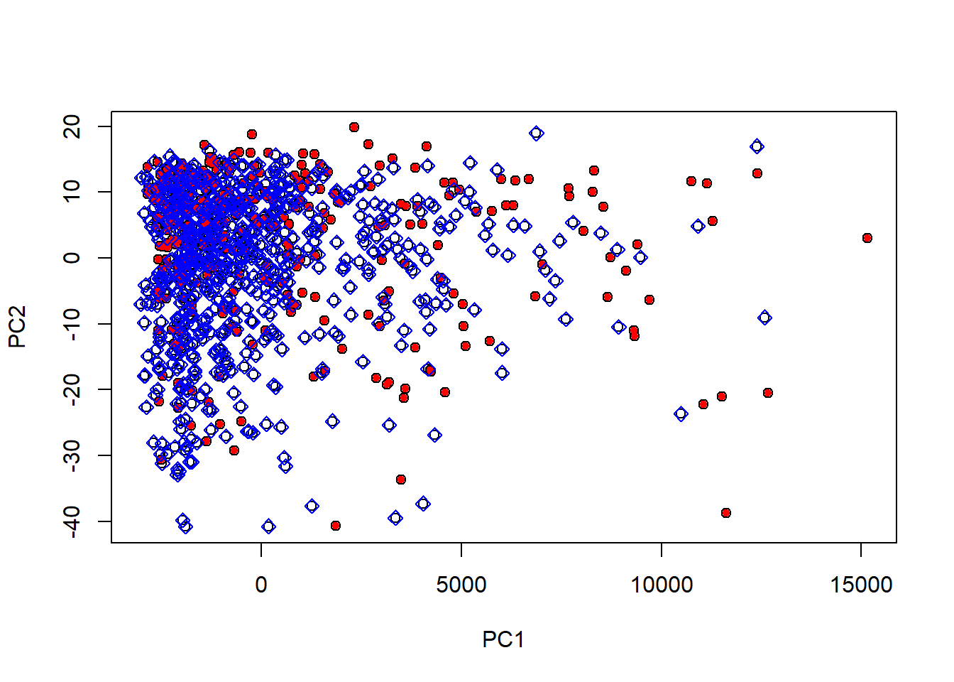
As we can see above, there isn’t a clear division between the class, which indicate that accuracy of Regression Tree is pretty reasonable.
Conclusion
Although the small numbers of observations, and the absence of a clearer division on the dataset classes, a simple Regression Tree (in sense of the generated tree model) proved capable to tackle the problem of making predictions on German Credit dataset.