By Salerno | March 19, 2020
1. Importing entire text files
# Open a file: file
file = open('c:/blogdown/moby_dick.txt', mode='r')

# Print it
print(file.read())

# Check whether file is closed
## CHAPTER 1. Loomings.
##
## Call me Ishmael. Some years ago--never mind how long precisely--having
## little or no money in my purse, and nothing particular to interest me on
## shore, I thought I would sail about a little and see the watery part of
## the world. It is a way I have of driving off the spleen and regulating
## the circulation. Whenever I find myself growing grim about the mouth;
## whenever it is a damp, drizzly November in my soul; whenever I find
## myself involuntarily pausing before coffin warehouses, and bringing up
## the rear of every funeral I meet; and especially whenever my hypos get
## such an upper hand of me, that it requires a strong moral principle to
## prevent me from deliberately stepping into the street, and methodically
## knocking people's hats off--then, I account it high time to get to sea
## as soon as I can. This is my substitute for pistol and ball. With a
## philosophical flourish Cato throws himself upon his sword; I quietly
## take to the ship. There is nothing surprising in this. If they but knew
## it, almost all men in their degree, some time or other, cherish very
## nearly the same feelings towards the ocean with me.print(file.closed)
# Close file## Falsefile.close()
# Check whether file is closed
print(file.closed)## True2. Importing text files line by line
# Read & print the first 3 lines
with open('c:/blogdown/moby_dick.txt') as file:
    print(file.readline())
    print(file.readline())
    print(file.readline())
## CHAPTER 1. Loomings.
##
##
##
## Call me Ishmael. Some years ago--never mind how long precisely--having3. Using NumPy to import flat files
# Import package
import numpy as np
import matplotlib.pyplot as plt

# Assign filename to variable: file
file = 'c:/blogdown/mnist_kaggle_some_rows.csv'

# Load file as array: digits
digits = np.loadtxt(file, delimiter=',')

# Print datatype of digits
print(type(digits))

# Select and reshape a row
## <class 'numpy.ndarray'>im = digits[21, 1:]
im_sq = np.reshape(im, (28, 28))
# Plot reshaped data (matplotlib.pyplot already loaded as plt)
plt.imshow(im_sq, cmap='Greys', interpolation='nearest')
plt.show()
## Traceback (most recent call last):
##   File "C:\ProgramData\Anaconda3\lib\site-packages\matplotlib\backends\backend_qt5.py", line 508, in _draw_idle
##     self.draw()
##   File "C:\ProgramData\Anaconda3\lib\site-packages\matplotlib\backends\backend_agg.py", line 388, in draw
##     self.figure.draw(self.renderer)
##   File "C:\ProgramData\Anaconda3\lib\site-packages\matplotlib\artist.py", line 38, in draw_wrapper
##     return draw(artist, renderer, *args, **kwargs)
##   File "C:\ProgramData\Anaconda3\lib\site-packages\matplotlib\figure.py", line 1709, in draw
##     renderer, self, artists, self.suppressComposite)
##   File "C:\ProgramData\Anaconda3\lib\site-packages\matplotlib\image.py", line 135, in _draw_list_compositing_images
##     a.draw(renderer)
##   File "C:\ProgramData\Anaconda3\lib\site-packages\matplotlib\artist.py", line 38, in draw_wrapper
##     return draw(artist, renderer, *args, **kwargs)
##   File "C:\ProgramData\Anaconda3\lib\site-packages\matplotlib\axes\_base.py", line 2607, in draw
##     self._update_title_position(renderer)
##   File "C:\ProgramData\Anaconda3\lib\site-packages\matplotlib\axes\_base.py", line 2548, in _update_title_position
##     ax.xaxis.get_ticks_position() in choices):
##   File "C:\ProgramData\Anaconda3\lib\site-packages\matplotlib\axis.py", line 2146, in get_ticks_position
##     self._get_ticks_position()]
##   File "C:\ProgramData\Anaconda3\lib\site-packages\matplotlib\axis.py", line 1833, in _get_ticks_position
##     minor = self.minorTicks[0]
## IndexError: list index out of range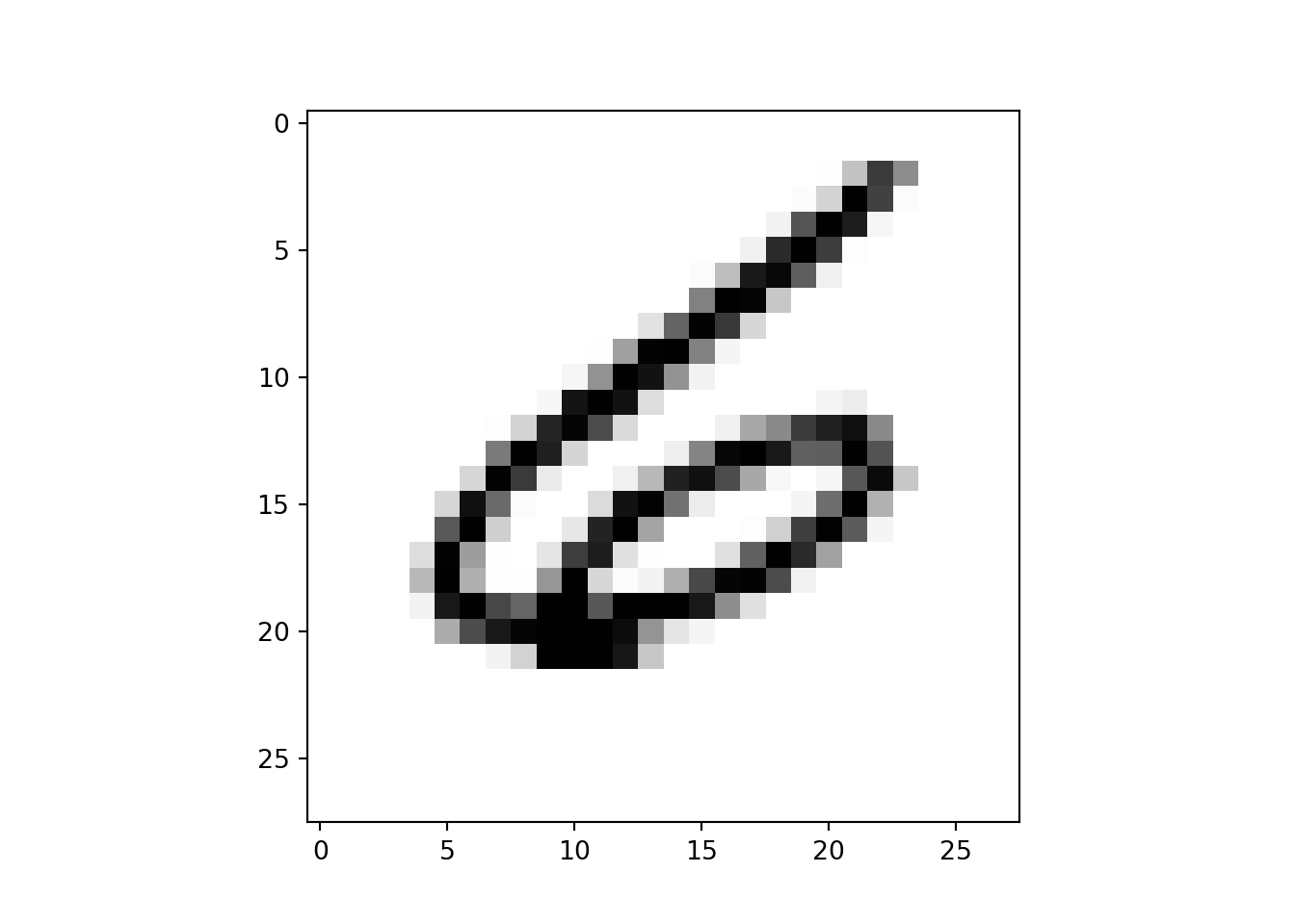
4. Customizing your NumPy import
# Assign filename: file
file = 'c:/blogdown/seaslug.txt'

# Import file: data
data = np.loadtxt(file, delimiter='\t', dtype=str)

# Print the first element of data
print(data[0])

# Import data as floats and skip the first row: data_float
## ['Time' 'Percent']data_float = np.loadtxt(file, delimiter='\t', dtype=float, skiprows=1)
# Print the 10th element of data_float
print(data_float[9])
# Plot a scatterplot of the data## [0. 0.357]plt.scatter(data_float[:, 0], data_float[:, 1])
plt.xlabel('time (min.)')
plt.ylabel('percentage of larvae')
plt.show()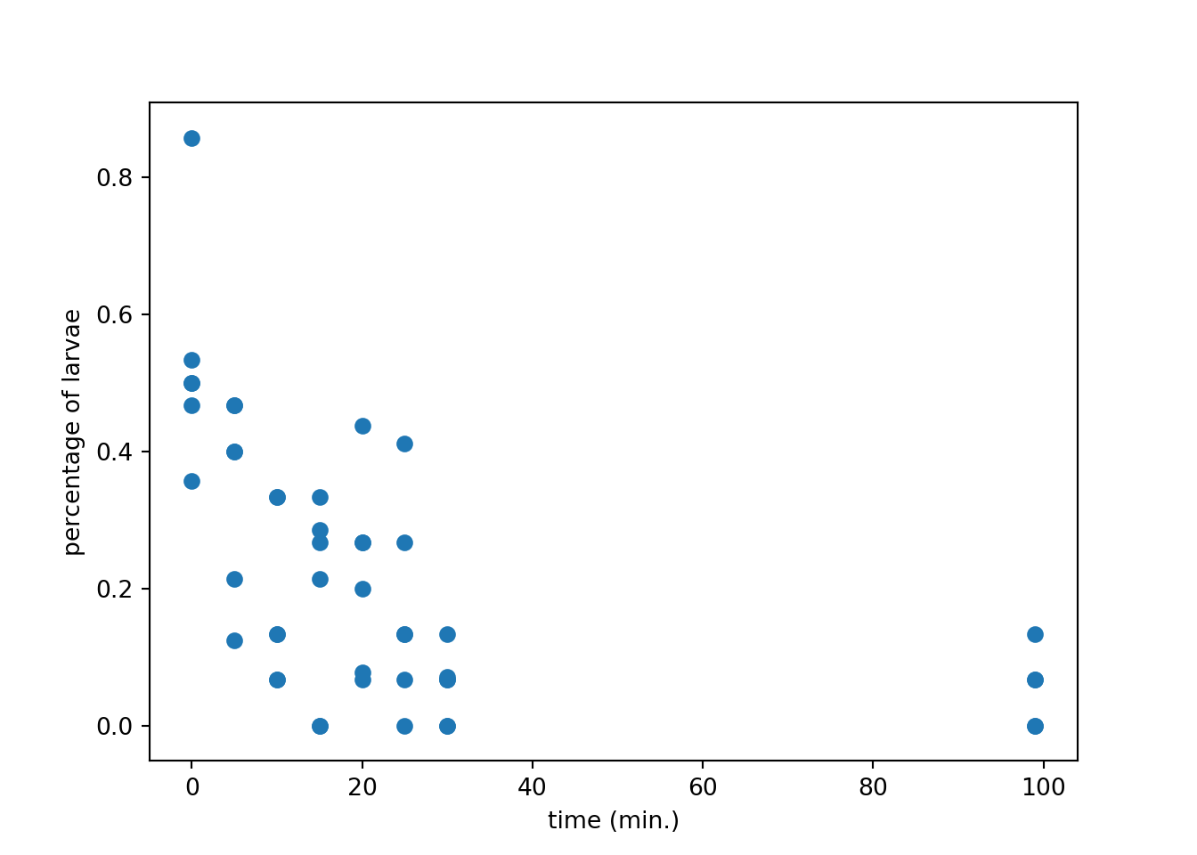
5. Working with mixed datatypes
data = 'c:/blogdown/titanic_sub.csv'

data = np.genfromtxt(data, delimiter=',', names=True, dtype=None)
## C:/ProgramData/Anaconda3/python.exe:1: VisibleDeprecationWarning: Reading unicode strings without specifying the encoding argument is deprecated. Set the encoding, use None for the system default.np.shape(data)## (891,)print(data['Fare'])## [ 7.25 71.2833 7.925 53.1 8.05 8.4583 51.8625 21.075
## 11.1333 30.0708 16.7 26.55 8.05 31.275 7.8542 16.
## 29.125 13. 18. 7.225 26. 13. 8.0292 35.5
## 21.075 31.3875 7.225 263. 7.8792 7.8958 27.7208 146.5208
## 7.75 10.5 82.1708 52. 7.2292 8.05 18. 11.2417
## 9.475 21. 7.8958 41.5792 7.8792 8.05 15.5 7.75
## 21.6792 17.8 39.6875 7.8 76.7292 26. 61.9792 35.5
## 10.5 7.2292 27.75 46.9 7.2292 80. 83.475 27.9
## 27.7208 15.2458 10.5 8.1583 7.925 8.6625 10.5 46.9
## 73.5 14.4542 56.4958 7.65 7.8958 8.05 29. 12.475
## 9. 9.5 7.7875 47.1 10.5 15.85 34.375 8.05
## 263. 8.05 8.05 7.8542 61.175 20.575 7.25 8.05
## 34.6542 63.3583 23. 26. 7.8958 7.8958 77.2875 8.6542
## 7.925 7.8958 7.65 7.775 7.8958 24.15 52. 14.4542
## 8.05 9.825 14.4583 7.925 7.75 21. 247.5208 31.275
## 73.5 8.05 30.0708 13. 77.2875 11.2417 7.75 7.1417
## 22.3583 6.975 7.8958 7.05 14.5 26. 13. 15.0458
## 26.2833 53.1 9.2167 79.2 15.2458 7.75 15.85 6.75
## 11.5 36.75 7.7958 34.375 26. 13. 12.525 66.6
## 8.05 14.5 7.3125 61.3792 7.7333 8.05 8.6625 69.55
## 16.1 15.75 7.775 8.6625 39.6875 20.525 55. 27.9
## 25.925 56.4958 33.5 29.125 11.1333 7.925 30.6958 7.8542
## 25.4667 28.7125 13. 0. 69.55 15.05 31.3875 39.
## 22.025 50. 15.5 26.55 15.5 7.8958 13. 13.
## 7.8542 26. 27.7208 146.5208 7.75 8.4042 7.75 13.
## 9.5 69.55 6.4958 7.225 8.05 10.4625 15.85 18.7875
## 7.75 31. 7.05 21. 7.25 13. 7.75 113.275
## 7.925 27. 76.2917 10.5 8.05 13. 8.05 7.8958
## 90. 9.35 10.5 7.25 13. 25.4667 83.475 7.775
## 13.5 31.3875 10.5 7.55 26. 26.25 10.5 12.275
## 14.4542 15.5 10.5 7.125 7.225 90. 7.775 14.5
## 52.5542 26. 7.25 10.4625 26.55 16.1 20.2125 15.2458
## 79.2 86.5 512.3292 26. 7.75 31.3875 79.65 0.
## 7.75 10.5 39.6875 7.775 153.4625 135.6333 31. 0.
## 19.5 29.7 7.75 77.9583 7.75 0. 29.125 20.25
## 7.75 7.8542 9.5 8.05 26. 8.6625 9.5 7.8958
## 13. 7.75 78.85 91.0792 12.875 8.85 7.8958 27.7208
## 7.2292 151.55 30.5 247.5208 7.75 23.25 0. 12.35
## 8.05 151.55 110.8833 108.9 24. 56.9292 83.1583 262.375
## 26. 7.8958 26.25 7.8542 26. 14. 164.8667 134.5
## 7.25 7.8958 12.35 29. 69.55 135.6333 6.2375 13.
## 20.525 57.9792 23.25 28.5 153.4625 18. 133.65 7.8958
## 66.6 134.5 8.05 35.5 26. 263. 13. 13.
## 13. 13. 13. 16.1 15.9 8.6625 9.225 35.
## 7.2292 17.8 7.225 9.5 55. 13. 7.8792 7.8792
## 27.9 27.7208 14.4542 7.05 15.5 7.25 75.25 7.2292
## 7.75 69.3 55.4417 6.4958 8.05 135.6333 21.075 82.1708
## 7.25 211.5 4.0125 7.775 227.525 15.7417 7.925 52.
## 7.8958 73.5 46.9 13. 7.7292 12. 120. 7.7958
## 7.925 113.275 16.7 7.7958 7.8542 26. 10.5 12.65
## 7.925 8.05 9.825 15.85 8.6625 21. 7.75 18.75
## 7.775 25.4667 7.8958 6.8583 90. 0. 7.925 8.05
## 32.5 13. 13. 24.15 7.8958 7.7333 7.875 14.4
## 20.2125 7.25 26. 26. 7.75 8.05 26.55 16.1
## 26. 7.125 55.9 120. 34.375 18.75 263. 10.5
## 26.25 9.5 7.775 13. 8.1125 81.8583 19.5 26.55
## 19.2583 30.5 27.75 19.9667 27.75 89.1042 8.05 7.8958
## 26.55 51.8625 10.5 7.75 26.55 8.05 38.5 13.
## 8.05 7.05 0. 26.55 7.725 19.2583 7.25 8.6625
## 27.75 13.7917 9.8375 52. 21. 7.0458 7.5208 12.2875
## 46.9 0. 8.05 9.5875 91.0792 25.4667 90. 29.7
## 8.05 15.9 19.9667 7.25 30.5 49.5042 8.05 14.4583
## 78.2667 15.1 151.55 7.7958 8.6625 7.75 7.6292 9.5875
## 86.5 108.9 26. 26.55 22.525 56.4958 7.75 8.05
## 26.2875 59.4 7.4958 34.0208 10.5 24.15 26. 7.8958
## 93.5 7.8958 7.225 57.9792 7.2292 7.75 10.5 221.7792
## 7.925 11.5 26. 7.2292 7.2292 22.3583 8.6625 26.25
## 26.55 106.425 14.5 49.5 71. 31.275 31.275 26.
## 106.425 26. 26. 13.8625 20.525 36.75 110.8833 26.
## 7.8292 7.225 7.775 26.55 39.6 227.525 79.65 17.4
## 7.75 7.8958 13.5 8.05 8.05 24.15 7.8958 21.075
## 7.2292 7.8542 10.5 51.4792 26.3875 7.75 8.05 14.5
## 13. 55.9 14.4583 7.925 30. 110.8833 26. 40.125
## 8.7125 79.65 15. 79.2 8.05 8.05 7.125 78.2667
## 7.25 7.75 26. 24.15 33. 0. 7.225 56.9292
## 27. 7.8958 42.4 8.05 26.55 15.55 7.8958 30.5
## 41.5792 153.4625 31.275 7.05 15.5 7.75 8.05 65.
## 14.4 16.1 39. 10.5 14.4542 52.5542 15.7417 7.8542
## 16.1 32.3208 12.35 77.9583 7.8958 7.7333 30. 7.0542
## 30.5 0. 27.9 13. 7.925 26.25 39.6875 16.1
## 7.8542 69.3 27.9 56.4958 19.2583 76.7292 7.8958 35.5
## 7.55 7.55 7.8958 23. 8.4333 7.8292 6.75 73.5
## 7.8958 15.5 13. 113.275 133.65 7.225 25.5875 7.4958
## 7.925 73.5 13. 7.775 8.05 52. 39. 52.
## 10.5 13. 0. 7.775 8.05 9.8417 46.9 512.3292
## 8.1375 76.7292 9.225 46.9 39. 41.5792 39.6875 10.1708
## 7.7958 211.3375 57. 13.4167 56.4958 7.225 26.55 13.5
## 8.05 7.7333 110.8833 7.65 227.525 26.2875 14.4542 7.7417
## 7.8542 26. 13.5 26.2875 151.55 15.2458 49.5042 26.55
## 52. 9.4833 13. 7.65 227.525 10.5 15.5 7.775
## 33. 7.0542 13. 13. 53.1 8.6625 21. 7.7375
## 26. 7.925 211.3375 18.7875 0. 13. 13. 16.1
## 34.375 512.3292 7.8958 7.8958 30. 78.85 262.375 16.1
## 7.925 71. 20.25 13. 53.1 7.75 23. 12.475
## 9.5 7.8958 65. 14.5 7.7958 11.5 8.05 86.5
## 14.5 7.125 7.2292 120. 7.775 77.9583 39.6 7.75
## 24.15 8.3625 9.5 7.8542 10.5 7.225 23. 7.75
## 7.75 12.475 7.7375 211.3375 7.2292 57. 30. 23.45
## 7.05 7.25 7.4958 29.125 20.575 79.2 7.75 26.
## 69.55 30.6958 7.8958 13. 25.9292 8.6833 7.2292 24.15
## 13. 26.25 120. 8.5167 6.975 7.775 0. 7.775
## 13. 53.1 7.8875 24.15 10.5 31.275 8.05 0.
## 7.925 37.0042 6.45 27.9 93.5 8.6625 0. 12.475
## 39.6875 6.95 56.4958 37.0042 7.75 80. 14.4542 18.75
## 7.2292 7.8542 8.3 83.1583 8.6625 8.05 56.4958 29.7
## 7.925 10.5 31. 6.4375 8.6625 7.55 69.55 7.8958
## 33. 89.1042 31.275 7.775 15.2458 39.4 26. 9.35
## 164.8667 26.55 19.2583 7.2292 14.1083 11.5 25.9292 69.55
## 13. 13. 13.8583 50.4958 9.5 11.1333 7.8958 52.5542
## 5. 9. 24. 7.225 9.8458 7.8958 7.8958 83.1583
## 26. 7.8958 10.5167 10.5 7.05 29.125 13. 30.
## 23.45 30. 7.75 ]6. Working with mixed datatypes (2)
data = 'c:/blogdown/titanic_sub.csv'

# Import file using np.recfromcsv: d
d = np.recfromcsv(data)

# Print out first three entries of d
## C:\ProgramData\Anaconda3\lib\site-packages\numpy\lib\npyio.py:2372: VisibleDeprecationWarning: Reading unicode strings without specifying the encoding argument is deprecated. Set the encoding, use None for the system default.
## output = genfromtxt(fname, **kwargs)print(d[:3])
## [(1, 0, 3, b'male', 22., 1, 0, b'A/5 21171',  7.25  , b'', b'S')
##  (2, 1, 1, b'female', 38., 1, 0, b'PC 17599', 71.2833, b'C85', b'C')
##  (3, 1, 3, b'female', 26., 0, 0, b'STON/O2. 3101282',  7.925 , b'', b'S')]
7. Using Pandas to import flatfiles as DataFrames
# Import pandas as pd
import pandas as pd

# Assign the filename: file
file = 'c:/blogdown/titanic_sub.csv'

# Read the file into a DataFrame: df
df = pd.read_csv(file)

# View the head of the DataFrame
print(df.head())
## PassengerId Survived Pclass ... Fare Cabin Embarked
## 0 1 0 3 ... 7.2500 NaN S
## 1 2 1 1 ... 71.2833 C85 C
## 2 3 1 3 ... 7.9250 NaN S
## 3 4 1 1 ... 53.1000 C123 S
## 4 5 0 3 ... 8.0500 NaN S
##
## [5 rows x 11 columns]type(df)
## <class 'pandas.core.frame.DataFrame'>8. Using pandas to import flat files as DataFrames (2)
# Assign the filename: file
file = 'c:/blogdown/titanic_sub.csv'

# Read the first 5 rows of the file into a DataFrame: data
data = pd.read_csv(file, nrows=5, header=None)

# Build a numpy array from the DataFrame: data_array
data_array = np.array(data)

# Print the datatype of data_array to the shell
print(type(data_array))
## <class 'numpy.ndarray'>9. Customizing your pandas import
# Import matplotlib.pyplot as plt
import matplotlib.pyplot as plt
# Assign filename: file
file = 'c:/blogdown/titanic_corrupt.txt'
# Import file: data
data = pd.read_csv(file, sep='\t', comment='#', na_values='Nothing')
# Print the head of the DataFrame
print(data.head())
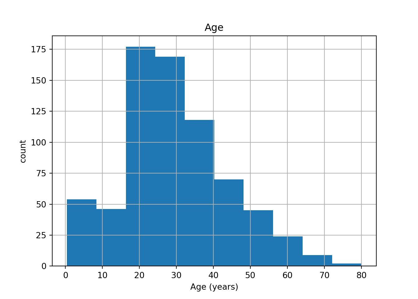
# Plot 'Age' variable in a histogram## PassengerId Survived Pclass ... Fare Cabin Embarked
## 0 1 0 3 ... 7.2500 NaN S #dfafdad
## 1 2 1 1 ... 71.2833 C85 C
## 2 3 1 3 ... 7.9250 NaN S
## 3 4 1 1 ... 53.1000 C123 S
## 4 5 0 3 ... 8.0500 NaN S
##
## [5 rows x 11 columns]pd.DataFrame.hist(data[['Age']])## array([[<matplotlib.axes._subplots.AxesSubplot object at 0x000000002025C248>]],
## dtype=object)plt.xlabel('Age (years)')
plt.ylabel('count')
plt.show()
10. Not so flat any more
import os
wd = os.getcwd()
os.listdir(wd)
## ['2015-07-23-r-rmarkdown.html', '2015-07-23-r-rmarkdown.Rmd', '2019-12-18-linear-regression.html', '2019-12-18-linear-regression.Rmd', '2019-12-19-data-frame.html', '2019-12-19-data-frame.Rmd', '2019-12-21-exponential-smoothing-model.html', '2019-12-21-exponential-smoothing-model.Rmd', '2019-12-23-r-packages-for-regression.html', '2019-12-23-r-packages-for-regression.Rmd', '2019-12-23-random-forest.html', '2019-12-23-random-forest.Rmd', '2019-12-27-quicksort-algorithm.html', '2019-12-27-quicksort-algorithm.Rmd', '2019-12-28-binary-search.html', '2019-12-28-binary-search.Rmd', '2020-01-05-knn-algorithm.html', '2020-01-05-knn-algorithm.Rmd', '2020-01-13-classifying-using-logistic-regression.html', '2020-01-13-classifying-using-logistic-regression.Rmd', '2020-01-19-correlation-and-regression.html', '2020-01-19-correlation-and-regression.Rmd', '2020-02-07-german-credit-and-regression-tree.html', '2020-02-07-german-credit-and-regression-tree.Rmd', '2020-02-29-a-game-of-chance.html', '2020-02-29-a-game-of-chance.Rmd', '2020-03-01-functions.html', '2020-03-01-functions.Rmd', '2020-03-09-iterables-versus-iterators.html', '2020-03-09-iterables-versus-iterators.Rmd', '2020-03-14-linear-models-scikit-learn.html', '2020-03-14-linear-models-scikit-learn.Rmd', '2020-03-14-tensorflow-2-quickstart-for-beginners.html', '2020-03-14-tensorflow-2-quickstart-for-beginners.Rmd', '2020-03-15-python-data-science-part-1.html', '2020-03-15-python-data-science-part-1.Rmd', '2020-03-18-supervised-learning-with-scikit-learn.html', '2020-03-18-supervised-learning-with-scikit-learn.Rmd', '2020-03-19-introduction-to-importing-data-in-python.html', '2020-03-19-introduction-to-importing-data-in-python.Rmd', '2020-03-19-introduction-to-importing-data-in-python_files', 'Chinook.sqlite', 'creating-a-new-theme.md', 'go-is-for-lovers.md', 'heart-disease-uci.zip', 'heart.csv', 'hugo-is-for-lovers.md', 'linked-post.md', 'migrate-from-jekyll.md', 'Northwind.sqlite', '_book', '_bookdown_files']11. Listing sheets in Excel files
# Import pandas
import pandas as pd

# Assign spreadsheet filename: file
file = 'c:/blogdown/battledeath.xlsx'

# Load spreadsheet: xls
xls = pd.ExcelFile(file)

# Print sheet names
print(xls.sheet_names)
## ['2002', '2004']12. Importing sheets from Excel files
# Assign spreadsheet filename: file
file = 'c:/blogdown/battledeath.xlsx'

# Load spreadsheet: xls
xls = pd.ExcelFile(file)

# Load a sheet into a DataFrame by name: df1
file1 = xls.parse('2004')

# Print the head of the DataFrame df1
print(file1.head())

# Load a sheet into a DataFrame by index: df2
## War(country) 2004
## 0 Afghanistan 9.451028
## 1 Albania 0.130354
## 2 Algeria 3.407277
## 3 Andorra 0.000000
## 4 Angola 2.597931file2 = xls.parse(0)
# Print the head of the DataFrame df2
print(file2.head())## War, age-adjusted mortality due to 2002
## 0 Afghanistan 36.083990
## 1 Albania 0.128908
## 2 Algeria 18.314120
## 3 Andorra 0.000000
## 4 Angola 18.96456013. Customizing your spreadsheet import
# Assign spreadsheet filename: file
file = 'c:/blogdown/battledeath.xlsx'

# Load spreadsheet: xls
xls = pd.ExcelFile(file)

# Parse the first sheet and rename the columns: df1
df1 = xls.parse(0, skiprows=1, names=('Country', 'AAM due to War (2002)'))

# Print the head of the DataFrame df1
print(df1.head())

# Parse the first column of the second sheet and rename the column: df2
## Country AAM due to War (2002)
## 0 Albania 0.128908
## 1 Algeria 18.314120
## 2 Andorra 0.000000
## 3 Angola 18.964560
## 4 Antigua and Barbuda 0.000000df2 = xls.parse(1, usecols=[0], skiprows=[0], names=['Country'])
# Print the head of the DataFrame df2
print(df2.head())
##                Country
## 0              Albania
## 1              Algeria
## 2              Andorra
## 3               Angola
## 4  Antigua and Barbuda
14. Importing SAS files
# Import sas7bdat package
from sas7bdat import SAS7BDAT

# Save file to a DataFrame: df_sas
with SAS7BDAT('c:/blogdown/sales.sas7bdat') as file:
    df_sas = file.to_data_frame()

# Print head of DataFrame
print(df_sas.head())

# Plot histogram of DataFrame features (pandas and pyplot already imported)
## YEAR P S
## 0 1950.0 12.9 181.899994
## 1 1951.0 11.9 245.000000
## 2 1952.0 10.7 250.199997
## 3 1953.0 11.3 265.899994
## 4 1954.0 11.2 248.500000pd.DataFrame.hist(df_sas[['P']])## array([[<matplotlib.axes._subplots.AxesSubplot object at 0x000000002C1DBB88>]],
## dtype=object)plt.ylabel('count')
plt.show()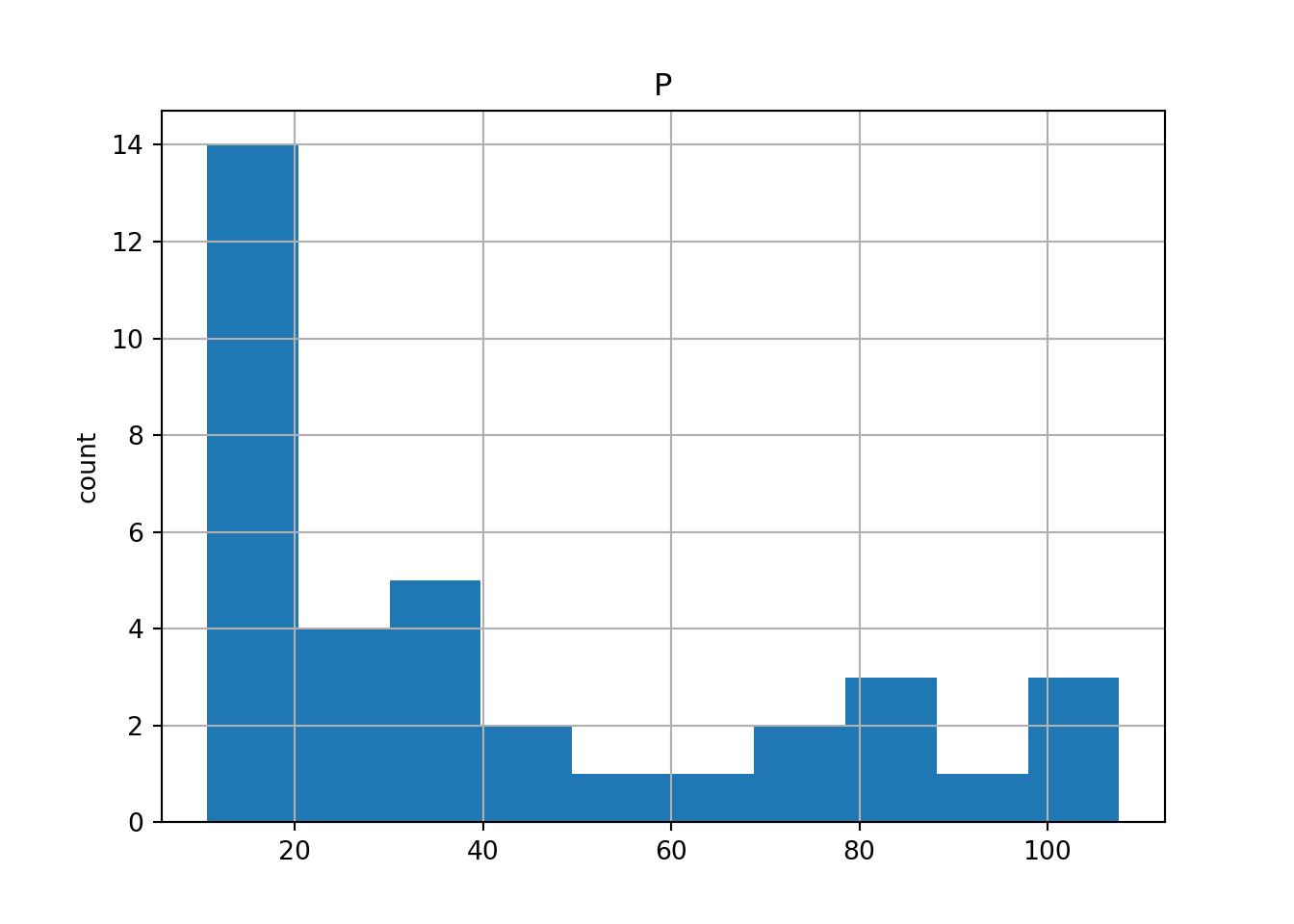
15. Importing Stata files
# Import pandas
import pandas as pd

# Load Stata file into a pandas DataFrame: df
df = pd.read_stata('c:/blogdown/disarea.dta')

# Print the head of the DataFrame df
print(df.head())

# Plot histogram of one column of the DataFrame
## wbcode country disa1 disa2 ... disa22 disa23 disa24 disa25
## 0 AFG Afghanistan 0.00 0.00 ... 0.00 0.02 0.00 0.00
## 1 AGO Angola 0.32 0.02 ... 0.99 0.98 0.61 0.00
## 2 ALB Albania 0.00 0.00 ... 0.00 0.00 0.00 0.16
## 3 ARE United Arab Emirates 0.00 0.00 ... 0.00 0.00 0.00 0.00
## 4 ARG Argentina 0.00 0.24 ... 0.00 0.01 0.00 0.11
##
## [5 rows x 27 columns]pd.DataFrame.hist(df[['disa10']])## array([[<matplotlib.axes._subplots.AxesSubplot object at 0x000000002C1DB648>]],
## dtype=object)plt.xlabel('Extent of disease')
plt.ylabel('Number of countries')
plt.show()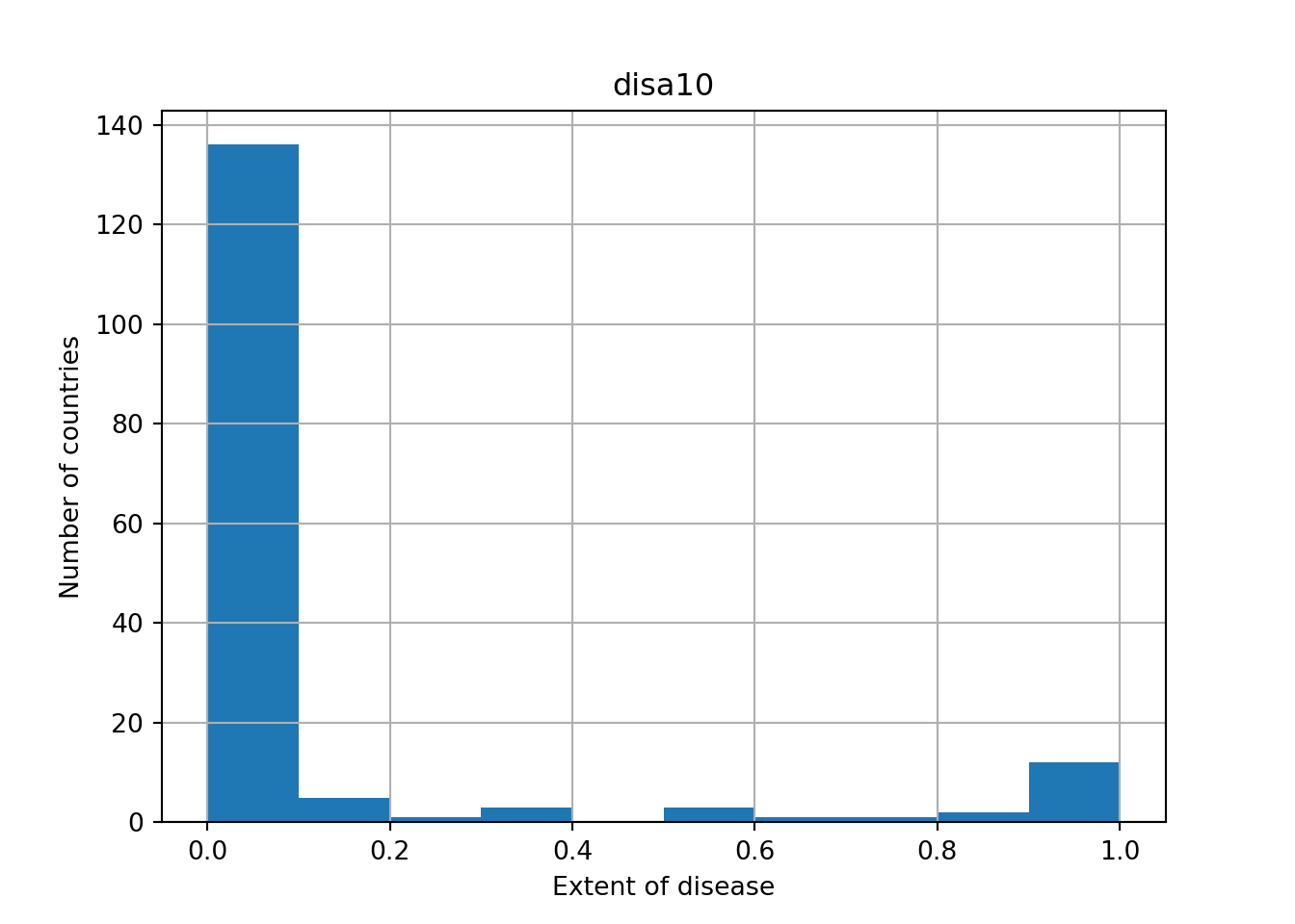
16. Using h5py to import HDF5 files
# Import packages
import numpy as np
import h5py

# Assign filename: file
file = 'c:/blogdown/L-L1_LOSC_4_V1-1126259446-32.hdf5'

# Load file: data
data = h5py.File(file, 'r')

# Print the datatype of the loaded file
print(type(data))

# Print the keys of the file
## <class 'h5py._hl.files.File'>for key in data.keys():
print(key)
## meta
## quality
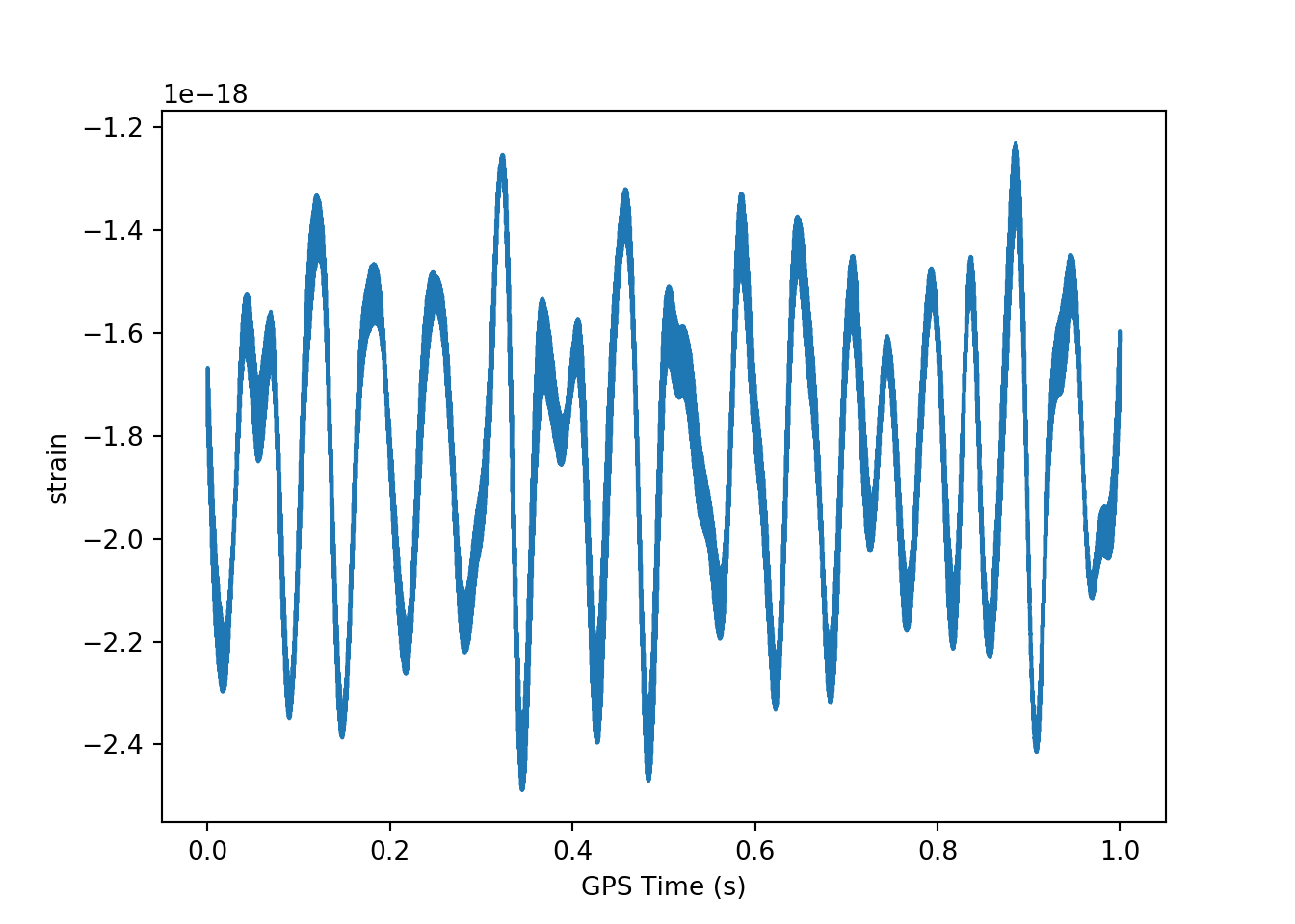
## strain17. Extracting data from your HDF5 file
# Import packages
import numpy as np
import h5py

# Assign filename: file
file = 'c:/blogdown/L-L1_LOSC_4_V1-1126259446-32.hdf5'

# Load file: data
data = h5py.File(file, 'r')


# Get the HDF5 group: group
group = data['strain']

# Check out keys of group
for key in group.keys():
    print(key)

# Set variable equal to time series data: strain
## Strainstrain = data['strain']['Strain'].value
# Set number of time points to sample: num_samples## C:/ProgramData/Anaconda3/python.exe:1: H5pyDeprecationWarning: dataset.value has been deprecated. Use dataset[()] instead.num_samples = 10000
# Set time vector
time = np.arange(0, 1, 1/num_samples)
# Plot data
plt.plot(time, strain[:num_samples])
plt.xlabel('GPS Time (s)')
plt.ylabel('strain')
plt.show()
18. Loading .mat files
# Import package
import scipy.io

# Load MATLAB file: mat
mat = scipy.io.loadmat('c:/blogdown/albeck_gene_expression.mat')

# Print the datatype type of mat
print(type(mat))
## <class 'dict'>19. The structure of .mat in Python
import scipy.io
import matplotlib.pyplot as plt
import numpy as np


# Load MATLAB file: mat
mat = scipy.io.loadmat('c:/blogdown/albeck_gene_expression.mat')

# Print the keys of the MATLAB dictionary
print(mat.keys())

# Print the type of the value corresponding to the key 'CYratioCyt'
## dict_keys(['__header__', '__version__', '__globals__', 'rfpCyt', 'rfpNuc', 'cfpNuc', 'cfpCyt', 'yfpNuc', 'yfpCyt', 'CYratioCyt'])print(type(mat['CYratioCyt']))
# Print the shape of the value corresponding to the key 'CYratioCyt'## <class 'numpy.ndarray'>print(mat['CYratioCyt'].shape)
# Subset the array and plot it## (200, 137)data = mat['CYratioCyt'][25, 5:]
fig = plt.figure()
plt.plot(data)
plt.xlabel('time (min.)')
plt.ylabel('normalized fluorescence (measure of expression)')
plt.show()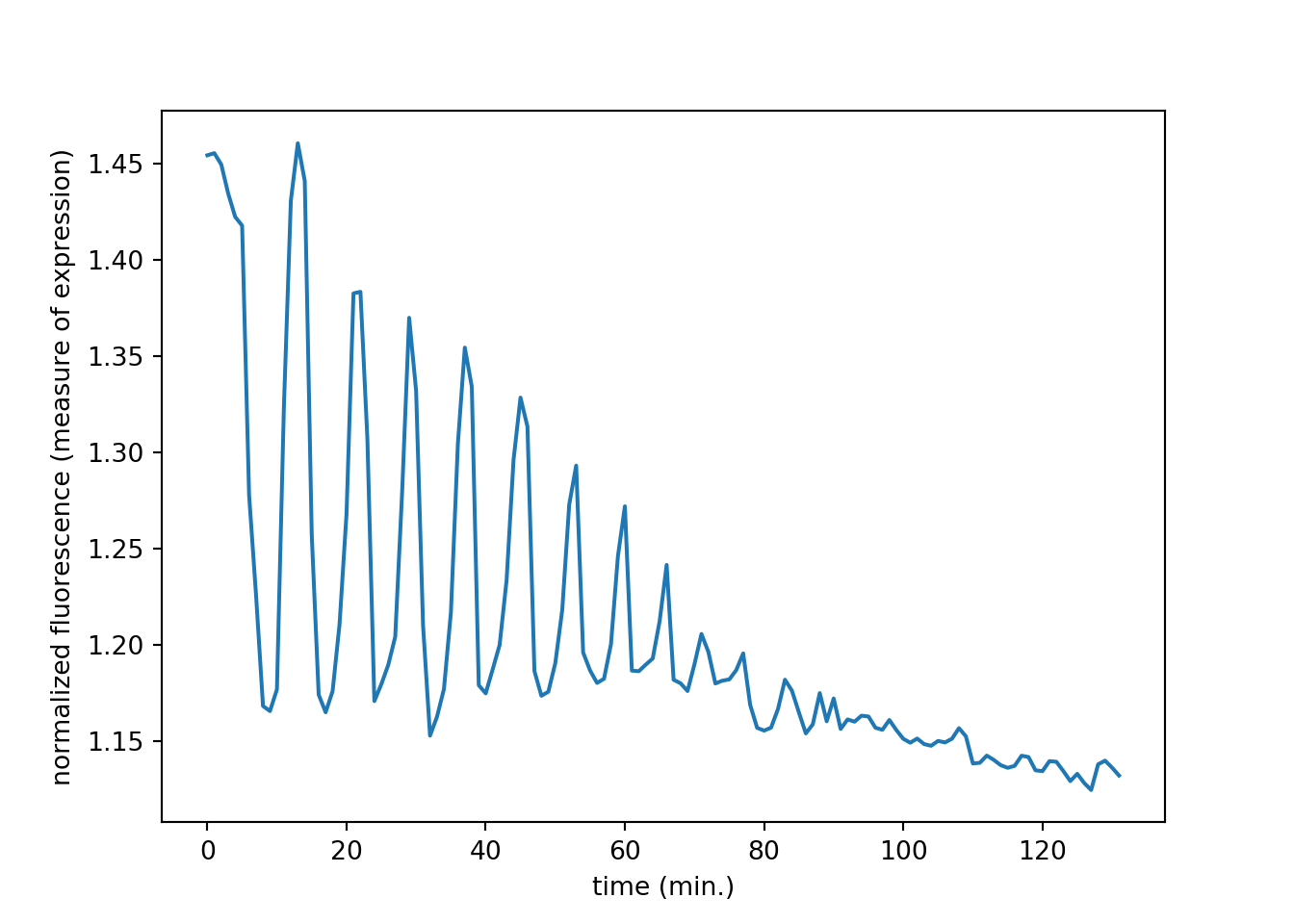
20. Creating a database engine
# Import necessary module
from sqlalchemy import create_engine

file = 'sqlite:///c:/blogdown/Chinook.sqlite'

# Create engine: engine
engine = create_engine(file)

table_names = engine.table_names()
print(table_names)
## ['Album', 'Artist', 'Customer', 'Employee', 'Genre', 'Invoice', 'InvoiceLine', 'MediaType', 'Playlist', 'PlaylistTrack', 'Track']21. The Hello World of SQL Queries!
# Import packages
from sqlalchemy import create_engine
import pandas as pd

file = 'sqlite:///c:/blogdown/Chinook.sqlite'

# Create engine: engine
engine = create_engine(file)

# Open engine connection: con
con = engine.connect()

# Perform query: rs
rs = con.execute('SELECT * FROM Album')

# Save results of the query to DataFrame: df
df = pd.DataFrame(rs.fetchall())

# Close connection
con.close()

# Print head of DataFrame df
print(df.head())
##    0                                      1  2
## 0  1  For Those About To Rock We Salute You  1
## 1  2                      Balls to the Wall  2
## 2  3                      Restless and Wild  2
## 3  4                      Let There Be Rock  1
## 4  5                               Big Ones  3
22. Customizing the Hello World of SQL Queries
# Import packages
from sqlalchemy import create_engine
import pandas as pd

file = 'sqlite:///c:/blogdown/Chinook.sqlite'

# Create engine: engine
engine = create_engine(file)

# Open engine in context manager
# Perform query and save results to DataFrame: df
with engine.connect() as con:
    rs = con.execute("SELECT LastName, Title FROM Employee")
    df = pd.DataFrame(rs.fetchmany(size=3))
    df.columns = rs.keys()

# Print the length of the DataFrame df
print(len(df))

# Print the head of the DataFrame df
## 3print(df.head())
##   LastName                Title
## 0    Adams      General Manager
## 1  Edwards        Sales Manager
## 2  Peacock  Sales Support Agent
23. Filtering your database records using SQL’s WHERE
# Import packages
from sqlalchemy import create_engine
import pandas as pd

file = 'sqlite:///c:/blogdown/Chinook.sqlite'

# Create engine: engine
engine = create_engine(file)

# Open engine in context manager
# Perform query and save results to DataFrame: df
with engine.connect() as con:
    rs = con.execute("SELECT * FROM Employee WHERE EmployeeId >= 6")
    df = pd.DataFrame(rs.fetchall())
    df.columns = rs.keys()

# Print the head of the DataFrame df
print(df.head())
## EmployeeId LastName ... Fax Email
## 0 6 Mitchell ... +1 (403) 246-9899 michael@chinookcorp.com
## 1 7 King ... +1 (403) 456-8485 robert@chinookcorp.com
## 2 8 Callahan ... +1 (403) 467-8772 laura@chinookcorp.com
##
## [3 rows x 15 columns]24. Ordering your SQL records with ORDER BY
# Import packages
from sqlalchemy import create_engine
import pandas as pd

file = 'sqlite:///c:/blogdown/Chinook.sqlite'

# Create engine: engine
engine = create_engine(file)

# Open engine in context manager
with engine.connect() as con:
    rs = con.execute("SELECT * FROM Employee ORDER BY BirthDate")
    df = pd.DataFrame(rs.fetchall())

    # Set the DataFrame's column names
    df.columns = rs.keys()

# Print head of DataFrame
print(df.head())
##    EmployeeId  LastName  ...                Fax                     Email
## 0           4      Park  ...  +1 (403) 263-4289  margaret@chinookcorp.com
## 1           2   Edwards  ...  +1 (403) 262-3322     nancy@chinookcorp.com
## 2           1     Adams  ...  +1 (780) 428-3457    andrew@chinookcorp.com
## 3           5   Johnson  ...   1 (780) 836-9543     steve@chinookcorp.com
## 4           8  Callahan  ...  +1 (403) 467-8772     laura@chinookcorp.com
##
## [5 rows x 15 columns]
25. Pandas and The Hello World of SQL Queries!
# Import packages
from sqlalchemy import create_engine
import pandas as pd

file = 'sqlite:///c:/blogdown/Chinook.sqlite'

# Create engine: engine
engine = create_engine(file)

# Execute query and store records in DataFrame: df
df = pd.read_sql_query("SELECT * FROM Album", engine)

# Print head of DataFrame
print(df.head())

# Open engine in context manager and store query result in df1
## AlbumId Title ArtistId
## 0 1 For Those About To Rock We Salute You 1
## 1 2 Balls to the Wall 2
## 2 3 Restless and Wild 2
## 3 4 Let There Be Rock 1
## 4 5 Big Ones 3with engine.connect() as con:
rs = con.execute("SELECT * FROM Album")
df1 = pd.DataFrame(rs.fetchall())
df1.columns = rs.keys()
# Confirm that both methods yield the same result
print(df.equals(df1))## True26. Pandas for more complex querying
# Import packages
from sqlalchemy import create_engine
import pandas as pd

file = 'sqlite:///c:/blogdown/Chinook.sqlite'

# Create engine: engine
engine = create_engine(file)


# Execute query and store records in DataFrame: df
df = pd.read_sql_query("SELECT * FROM Employee WHERE EmployeeId >= 6 ORDER BY BirthDate", engine)

# Print head of DataFrame
print(df.head())
##    EmployeeId  LastName  ...                Fax                    Email
## 0           8  Callahan  ...  +1 (403) 467-8772    laura@chinookcorp.com
## 1           7      King  ...  +1 (403) 456-8485   robert@chinookcorp.com
## 2           6  Mitchell  ...  +1 (403) 246-9899  michael@chinookcorp.com
##
## [3 rows x 15 columns]
27. The power of SQL lies in relationships between tables: INNER JOIN
# Import packages
from sqlalchemy import create_engine
import pandas as pd

file = 'sqlite:///c:/blogdown/Chinook.sqlite'

# Create engine: engine
engine = create_engine(file)

# Open engine in context manager
# Perform query and save results to DataFrame: df
with engine.connect() as con:
    rs = con.execute("SELECT Title, Name FROM Album INNER JOIN Artist on Album.ArtistID = Artist.ArtistID")
    df = pd.DataFrame(rs.fetchall())
    df.columns = rs.keys()

# Print head of DataFrame df
print(df.head())
##                                    Title       Name
## 0  For Those About To Rock We Salute You      AC/DC
## 1                      Balls to the Wall     Accept
## 2                      Restless and Wild     Accept
## 3                      Let There Be Rock      AC/DC
## 4                               Big Ones  Aerosmith
28. Filtering your INNER JOIN
# Import packages
from sqlalchemy import create_engine
import pandas as pd

file = 'sqlite:///c:/blogdown/Chinook.sqlite'

# Create engine: engine
engine = create_engine(file)

# Execute query and store records in DataFrame: df
df = pd.read_sql_query("SELECT * FROM PlaylistTrack INNER JOIN Track on PlaylistTrack.TrackId = Track.TrackId WHERE Milliseconds < 250000", engine)

# Print head of DataFrame
print(df.head())
##    PlaylistId  TrackId  TrackId  ... Milliseconds    Bytes  UnitPrice
## 0           1     3390     3390  ...       217732  3559040       0.99
## 1           1     3392     3392  ...       230758  3766605       0.99
## 2           1     3393     3393  ...       218916  3577821       0.99
## 3           1     3394     3394  ...       228366  3728955       0.99
## 4           1     3395     3395  ...       213831  3497176       0.99
##
## [5 rows x 11 columns]
comments powered by Disqus